What is Expected from RDC?

First uploaded on 2022/09/19
Last updated on 2024/11/22
Copyright(C)2022-2023 jos <jos@kaleidoscheme.com> All rights reserved.

[NOTE]
Reference figures resulting from the model calculations corresponding to each item will be added at random.

Our derivation and application of Radiatively Driven Circulation (RDC) theory were for a vertical two-dimensional equilibrium atmosphere. In this case, no dynamically forced flow effects, such as dynamical detrainment, were observed; instead, RDC was dominant in the mass/heat/water vapor transport around the cumulus. It seems to us that the application of RDC-based parameterization to the representation of three-dimensional time-developing atmospheric structure has more potential than continued improvements on existing dynamical detrainment. If we assume that the same results are obtained for the 3D atmosphere as for the 2D, we can expect the following results:

• The structure of the atmosphere produced by the cumulus-resolving model can be well produced by RDC alone ( Iwasa et al. 2002)． (Only the convective boundary layer region near the surface, which is dominated by convective process, has a different structure.)


• Because transport occurs in RDC from within the cumulus to outside the cumulus over the entire vertical extent of the troposphere, water vapor can be transported much more efficiently than by dynamical detrainment ( Iwasa et al. 2002)．


• For different horizontal distances between cumulus clouds, the RDC gives geometrically similar humidity distributions. This means that the vertical profile of horizontally averaged humidity is independent of the distance between cumulus clouds. This is because RDC is essentially solved as a boundary-value problem and thus has efficient transport capacity ( Iwasa et al. 2002)． (In the case of Dynamical Detrainment, it is very difficult to transport far when the distance between cumulus clouds is large.)
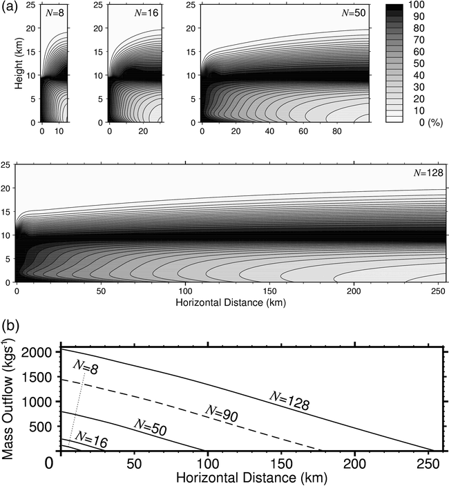  Figure WIEFR-1.
  Horizontal distance independence of KCM atmosphere:
  left and right ends of each figure are the centers of cumulus and subsidence, respectively.
  (a) Two-dimensional distributions of relative humidity obtained for different horizontal grid numbers N = 8, 16, 50, 128.
  (b) Horizontal profiles of the horizontal mass flux vertically integrated over the entire domain for the cases of N = 8, 16, 50, 90, 128.
  (Cited from Fig. F1 in Iwasa et al. 2002.)



• Against warming, the distribution of relative humidity in the troposphere is kept similar in RDC. Therefore RDC supports the validity of convective adjustment method based on the assumption of constant relative humidity in the troposphere. At the same time, this implies that the water vapor mixing ratio (absolute humidity) in the atmosphere increases rapidly with warming, because the saturated water vapor content increases rapidly with increasing temperature. This means that the water vapor feedback on warming is expected to be strongly positive ( Iwasa et al. 2004).


• In particular, the optical thickness versus the vertical structure of horizontally averaged atmospheric physics is unchanged for warming in our models. This implies that the troposphere, which is in radiative-convective equilibrium, is in fact strongly dominated by radiative process, suggesting the superiority of RDC over dynamical detrainment ( Iwasa et al. 2004)．
  
  Figure WIEFR-2.
  Vertical profiles of mean temperature vs mean optical depth at equilibrium from the DCM and KCM for the three warming scenarios. The analytic profile for radiative equilibrium (broken line) is also shown.
  In the range of optical depths less than 1.2, the profiles coincide with each other, not only in radiative equilibrium but also in radiative-convective equilibrium. In the region of larger optical depth corresponding to the convection-dominated convective boundary layer (CBL), the profiles diverge from each other.
  (Cited from Fig. 4 in Iwasa et al. 2004.)

1. in the vertical direction,
   because outflow occurs at all the altitudes trough the cumulus flank.
2. for different cumulus spacing so as to maintain the horizontally averaged relative humidity unchanged,
   because RDC is solved as a boundary-value problem.
3. for different warming condition,
   because the vertical structures of the atmosphere are the same if they are viewd with optical depth.

• Objects with strong optical properties in the atmosphere, such as clouds, have the potential to directly affect the RDC and alter the flow field. For example, in the middle troposphere near the melting level, where temperatures reach 0°C, optical properties change significantly in the vertical direction due to the phase change of water, causing significant outflow from the cumulus domain in the vicinity of this layer ( Iwasa et al. 2012)．


• Although this is not a direct result of RDC, the "subcloud-layer warming effect" should also be considered when discussing global warming: our DCM (Dynamical Convection Model), which explicitly treats convective motion, shows that the thickness of the convective boundary layer (CBL) generated at the bottom of the atmosphere increases with warming. This phenomenon further accelerates near-surface warming, because the temperature lapse rate takes within the CBL a dry adiabatic value, which is larger than the moist adiabatic lapse rate just above the CBL. This additional warming effect will be a very serious problem because human activity and the state of water at the Earth's surface are greatly affected by the temperature of the atmosphere near the surface ( Iwasa et al. 2004).
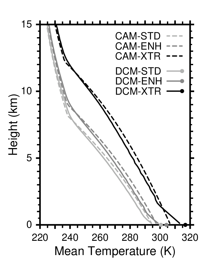  Figure WIEFR-4(a)
  Vertical profiles of the mean temperature obtained from the DCM (with the CBL, solid lines) for the STD, ENH, and XTR warming scenarios. The results obtained from the CAM (convective-adjustment model: without the CBL, broken lines) are also shown. (The relative humidity in the troposphere of the CAM was adjusted so as that the CAM provides the same bottom temperature for the STD scenario as the DCM.) You can see near the surface that the CBL with a dry adiabatic lapse rate, which is larger than the moist adiabatic lapse rate above it, is formed and its thickness is increasing with warming. (Salvaged from working files for Iwasa et al. 2004)．
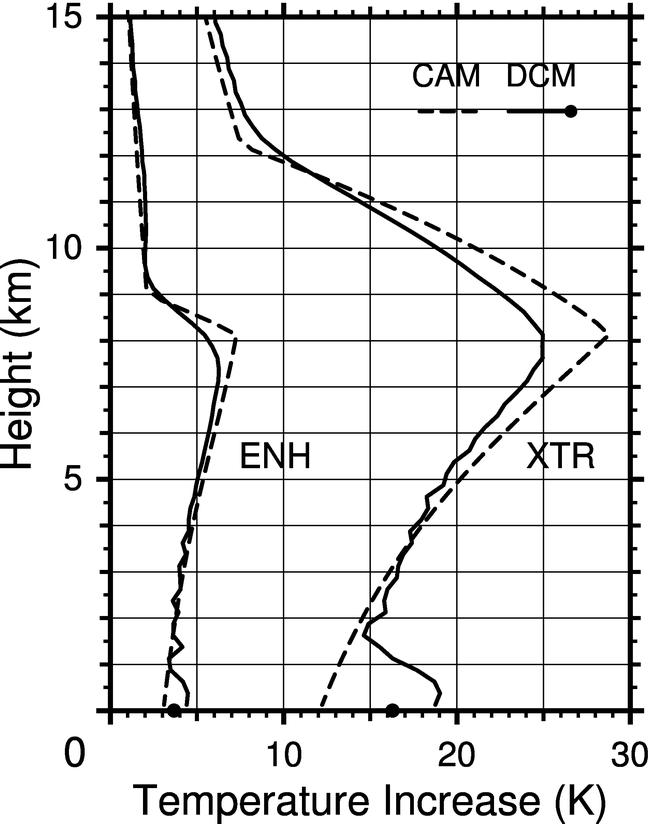  Figure WIEFR-4(b)
  Vertical profiles of the mean temperature INCREASE obtained from the DCM and CAM for the ENH and XTR warming scenarios compared to the STD scenario, respectively, calculated from the data shown in Fig. WIEFR-4(a). The temperature increase for each scenario is roughly the same between DCM and CAM, but the DCM, increasing the CBL thickness with warming, shows "subcloud-layer warming effect", an additional increase in temperature at the bottom of the atmosphere than the CAM for each senario. (Cited from Fig. 14 in Iwasa et al. 2004)．