[NOTE]
Time averaged temperature lapse rate <Γ>k on the layer at an altitude-index k can be calculated by dividing the negated difference in the time averaged temperature -Δ<T>k by the altitude difference Δzk, for example as \begin{equation} \begin{array}{ll} \displaystyle {\left< \Gamma \right>}_{k} & = & \displaystyle {\left[ - \frac{\partial \left< T \right>}{\partial z} \right]}_{k} \\ & = & \displaystyle - \frac {{\Delta \left< T \right>}_{k}} {{\Delta z}_{k}} \\ & = & \displaystyle - \frac {{\left< T \right>}_{k+1} -{\left< T \right>}_{k-1}} {{z}_{k+1}-{z}_{k-1}} \end{array} \nonumber \end{equation} using the values on the adjacent layers at the altitude-indexes k+1 and k-1 for an equally spaced vertical grid-point system. Of course, you can apply an appropriate differencing method depending on your model configuration.
[NOTE]
The negated z-derivative value on the right-hand side of Eq. (8') on the layer at an altitude-index k in the numerical model can be calculated by dividing the negated difference in the vertical mass flux -Δ(<ρ> wR)k by the altitude difference Δzk, for example as \begin{equation} \begin{array}{ll} \displaystyle {\left[ - \frac{\partial}{\partial z} \left( \left< \rho \right> {w}_{R} \right) \right]}_{k} & = & \displaystyle - \frac {{\Delta \left(\left< \rho \right> {w}_{R}\right)}_{k}} {{\Delta z}_{k}} \\ & = & - \displaystyle \frac {{\left(\left< \rho \right> {w}_{R}\right)}_{k+1} -{\left(\left< \rho \right> {w}_{R}\right)}_{k-1}} {{z}_{k+1}-{z}_{k-1}} \end{array} \nonumber \end{equation} using the values on the adjacent layers at the altitude-indexes k+1 and k-1 for an equally spaced vertical grid-point system. Of course, you can apply an appropriate differencing method depending on your model configuration. Thus, only arithmetic is necessary to check the sign of the value on the right-hand side of Eq. (8').
Congratulations! You have verified the presence of RDC in your model. You should proceed to a more rigorous RDC analysis in Suggested Development Steps for RDC Parameterization .
[NOTE]
The main reason why the atmospheric vertical mass flux <ρ>wR is a divergent field is the steep density stratification of the atmosphere, which has an exponential profile with respect to height z. Even when the radiatively driven subsidence velocity wR contains some vertical perturbations, multiplied by an atmospheric density <ρ> with a much larger vertical gradient, the atmospheric vertical mass flux <ρ>wR will be vertically divergent in general, especially when the clear sky occupies the outer area of the cumulus clouds as in the tropics and subtropics.
[NOTE]
You don't need to compute the detailed horizontal flow field (uR,vR) by solving the RDC equation (8') at this stage of simple verification. Identifying the negative value trend on the right-hand side of Eq. (8') outside the cumulus clouds is sufficient to guarantee the RDC outflow from the cumulus clouds.
[NOTE]
Don't look at the layers near the surface. As these are domains of the convective boundary layer (CBL), which is dominated by convection rather than radiation, RDC should not be observed here.
[NOTE]
A general image of the divergent subsidence mass flux <ρ>wR, which should be realized in the Earth's troposphere, is shown in Fig. 6 below. Because of the small subsidence mass flux in the upper layer and the large subsidence mass flux in the lower layer due to the strong density stratification in the atmosphere, the vertical flow alone would result in a mass-divergent field, creating a vacuum everywhere.
Confirming that the right-hand side of Eq. (8') is generally negative means that you have confirmed that the divergence field δ(<ρ>wR)/δz>0 for the vertical mass flux as shown in Fig. 6.
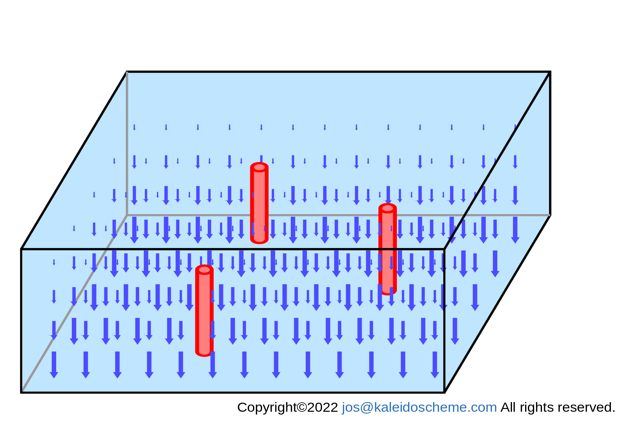
Schematic representation of the subsidence mass fluxes <ρ>wR (Eq. (3')) thermodynamically balanced with radiative cooling in the computational area. The subsidence mass flux is shown as a downward-pointing blue arrow at each computational grid-point in the atmosphere. The subsidence mass flux has small values in the upper layers and large values in the lower layers, resulting in a mass divergence field throughout the troposphere, which alone cannot sustain a flow field, because a vacuum is created everywhere in the troposphere.
A general image of the convergent horizontal mass flux (<ρ>uR,<ρ>vR) induced to compensate for the vacuum created by the divergent subsidence mass flux <ρ>wR above is shown in Fig. 8 below. This flux must be induced out of the cumulus domains, because they are the only source domains supplying mass/heat/water vapor in the troposphere.
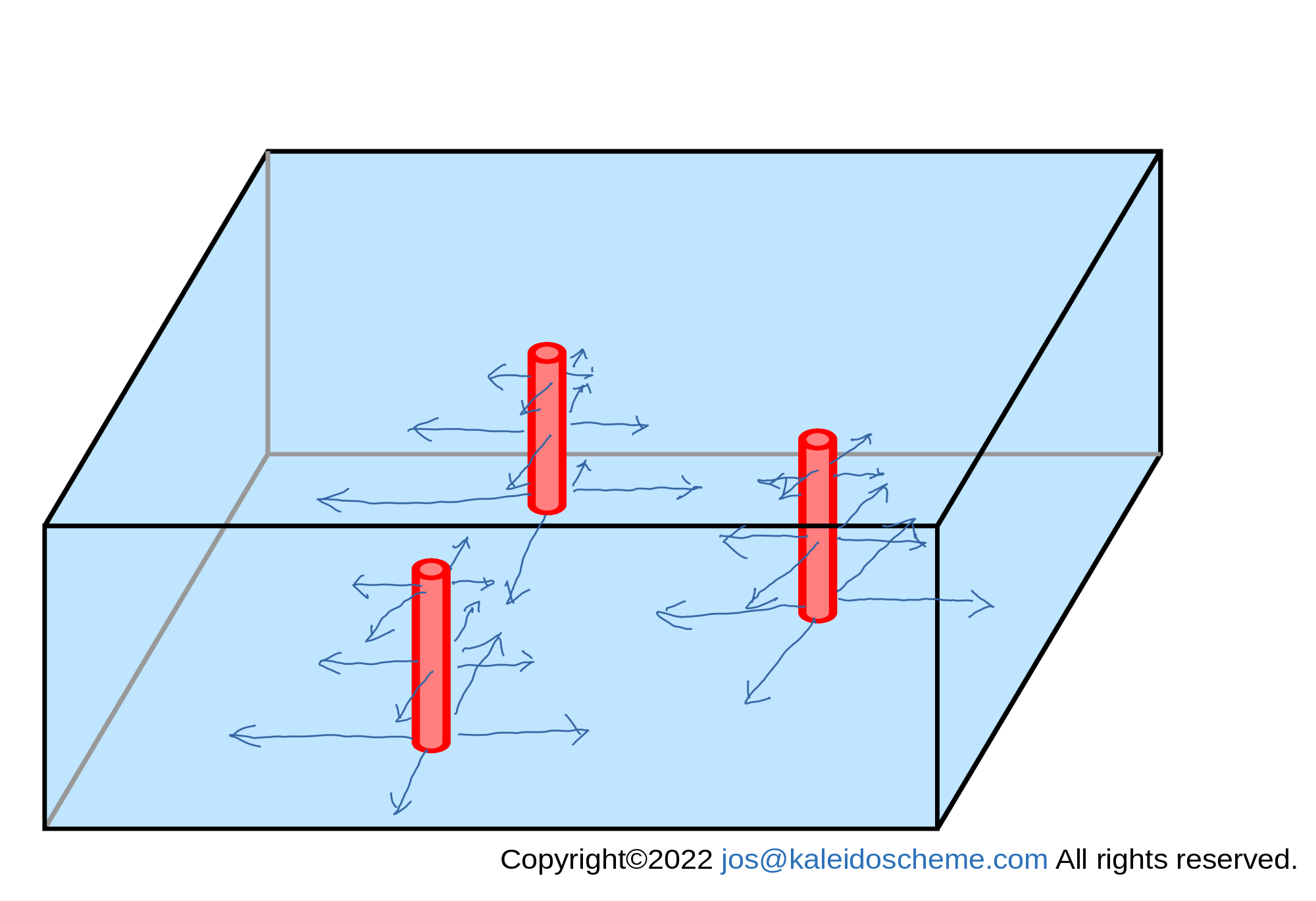
Convergent horizontal mass fluxes (<ρ>uR,<ρ>vR) induced outward from the supplying source (cumulus) domains to compensate for the divergence of the subsidence mass fluxes shown in Fig. 6.: the outgoing horizontal mass flux has a larger value closer to the supplying source domain and a smaller value away from it. Although the figure shows only a limited number of outflows, outflows actually occur in all argument directions around the supplying source domain.
Finally, the vertical <ρ>wR and horizontal (<ρ>uR,<ρ>vR) mass fluxes are combined to form the RDC flow field (<ρ>uR,<ρ>vR,<ρ>wR) as shown in Fig. 9 below.
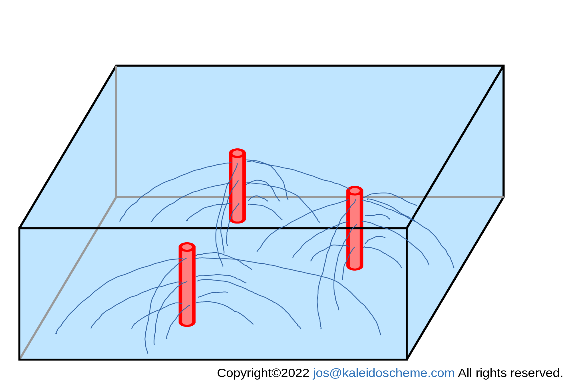
Conceptual streamlines of RDC around the supplying source domains, which are formed by the divergent subsidence mass flux <ρ>wR and the convergent horizontal mass flux (<ρ>uR,<ρ>vR) shown in Figs. 6 and 8, respectively. Although only a limited number of streamlines are shown in the figure, outflows actually occur in all argument directions around the supplying source domain.
Possible causes are
- If your model has already introduced a cumulus parameterization other than the RDC scheme, this check may not work correctly. This is because the cumulus parameterization you are currently using destroys the equilibrium state of the heat and continuity of the atmosphere outside the cumulus. In other words, you have proven that the parameterization is physically incorrect because it focuses too much on the internal dynamics of the cumulus and does not take into account its effect on the atmospheric structure outside the cumulus. Such a parameterization is not realistic. The current parameterization should be abandoned immediately and the RDC scheme adopted. (In a cumulus-resolving model, where there is no such artificial parameterization and all flows are based on physical laws, the RDC presence check should always succeed.)
- The model atmosphere is not in an equilibrium state. You should continue to run the model still further or change the initial state to a more appropriate one.
- Did you output data averaged over 10 hours? Instantaneous values do not allow us to see RDC due to perturbations in short time-space scales such as gravity waves. Depending on the model and the condition, it may be necessary to average over shorter or longer periods. The trend should be clearer if the average time is increased, for example, to 20 hours or 24 hours. Please experiment.
-
In procedure 3. above,
we made a very rough approximation by using the time-averaged value of <Γ>
directly in the first factor
(g/cp-Γ)-1
on the right-hand side of Eq.(3'),
which is the denominator.
Perhaps this approximation did not work well in your model
and you should use the time averaged value
<(g/cp-Γ)-1>
of the entire first factor
on the right-hand side of Eq. (3').
In this case you will need to add this time averaging calculation to your model code.
If it still does not show a clear trend, please perform the most rigorous check to see if the right-hand side value of Eq. (16'') \begin{eqnarray} \frac{{\partial}^{2} \Phi}{\partial {x}^{2}} + \frac{{\partial}^{2} \Phi}{\partial {y}^{2}} = \left< \frac{\partial}{\partial z} \left[ \rho {\left( \frac{g}{{c}_{p}} - \Gamma \right)}^{-1} {\left. \frac{\partial {T}}{\partial t} \right|}_{R} \right] \right> \hspace{1cm} \nonumber \end{eqnarray} shown in STEP-2: More Rigorous RDC Analysis becomes generally POSITIVE. - Very strong dynamic forcing may have obscured the flow of RDC. We are confident that the RDC will be present even in such a situation, but for now simple verification, it would be better to give it an atmospheric field that is a little easier to see. It is recommended to assume an atmospheric field at low latitudes, i.e., tropics and subtropics, that does not include mid- and high-latitude disturbances. This is the climatologically most important area and the area where RDC is most effective. The RDC will be simpler and you will have less chance of verification failures.
-
There may be optical objects in the atmosphere,
such as stratified clouds for example,
that significantly affect the radiative transfer.
This is not a false atmospheric field.
However,
it is our experience that in this case there can be strong local radiative cooling
near the top of the clouds,
or possibly net heating in the lower part of the clouds,
and then RDC causes a remarkable flow.
See
one of our reports.
As mentioned in the previous item, we recommend that when verifying the presence of RDC, the first step is to give conditions of the low-latitude atmosphere, where the outside of the cumulus tends to be clear sky.
The negative value trend on the right-hand side of Eq. (8') should be realized in the Earth's atmosphere. From our perspective, there is no atmosphere on Earth that does not have this essential characteristic. If such a model exists and claims to be able to represent the real atmosphere, we must question it. And if you still have trouble estimating the right-hand side of Eq. (8') in your model, please contact us. We will be happy to discuss with you, free of charge, why the simple RDC analysis does not work with your model.