-
Partitioning the Whole Horizontal Computational Area
into Presegmented Compartments
As will be explained on this page, RDC is solved as a boundary-value problem on the horizontal plane at each altitude. Provided that the full RDC flow is always realized, it is theoretically possible to calculate the RDC flow field for the entire horizontal area as it is. However, there are two reasons to partition the entire horizontal area into multiply presegmented compartments:
- The computational complexity for RDC boundary-value problem per run may be larger than that for dynamical detrainment. If the computational resource (CPU and memory) is not sufficient to cover the entire horizontal computational area, the partitioning will reduce the RDC calculation amount.
- As will be explained later, the full RDC flow may not always be realized in the model due to lack of mass flux in the supplying source (cumulus) domains. The partitioning will be needed for parameter tuning to limit the RDC mass flux within a compartment of its reach, depending on the method of limiting the RDC flow. (For example, the limiting method we propose below requires this partitioning, but of course there may be other methods.)
This partitioning is based on the distribution of radiation characteristics in the atmosphere. One example, as in Iwasa et al. (2012) (for a longitude-averaged latitude-altitude two-dimensional atmosphere), is to use the point of local minimum radiative cooling rate as the boundary between presegmented compartments. In a three-dimensional atmosphere, the boundaries of the compartments in the horizontal plane at each altitude will generally be curves defined as those of the troughs of the local minimum radiative cooling rates. In order to automatically perform such partitioning in a numerical model, pattern recognition techniques, such as those used to extract the contour of a photograph, may be used for the horizontal distribution of the radiative cooling rate.
The only criterion for defining a compartment that RDC can reach is the horizontal distribution of radiative cooling rates. The existence and number of supplying source domains for cumulus clouds and larger disturbances, which will be explained later, need not be taken into account when dividing a compartment. In other words, there may or may not be any number of supplying source domains in a single compartment.
[NOTE]
Regions closer to a cumulus cloud have a higher concentration of water vapor at the same altitude. Consequently, their optical thickness is greater and their radiative cooling rate is generally higher within the range of water vapor content in the Earth's atmosphere. In regions farthest reachable by RDC flow, on the other hand, the opposite condition prevails. Since the optical thickness is smaller there, the radiative cooling rate is generally lower. This is the physical significance of taking the region of locally-minimum radiative cooling rate as the boundary of the RDC reachable range.[NOTE]
Because it was tedious to create, there is no diagram showing an example of this partitioning. Therefore, it may be difficult for some readers to imagine this partitioning. For example, Iwasa et al. (2012) analyzed a longitudinally averaged 2D atmosphere, in which the RDC boundary value problem was solved with 25 degrees north latitude as the northernmost point where the RDC extends, based on the radiative cooling rate distribution. Because the RDC scheme shown here deals with a 3D atmosphere, the horizontal boundary of the RDC is generally a closed curve rather than a point. Nevertheless, the RDC boundary is again determined from the radiative cooling rate distribution.[NOTE]
This partitioning procedure is intended for cases where computer resources are not sufficient to solve the RDC boundary value problem for the entire given horizontal area. Therefore, when making a rough estimate of the full RDC flow ignoring the constraint imposed by the limited mass flux in the cumulus, this partitioning is not always necessary if such resources are sufficient. Similarly, if the given horizontal area is small, it is better to leave everything to the boundary value problem solver without partitioning. In any case, you don't need to worry about this partitioning until the final procedure of limiting constant value tuning is applied to RDC.[NOTE]
If this partitioning of the computational area is done, replace all references to "the calculation area" with "each presegmented compartment" in the following description. -
Designation of Supplying Source Domains
In general, in models that include parameterization, not all physical quantities are automatically computed in the model. They require external parameters. In RDC parameterization, we need to provide the "supplying source domains". The domains are the source for the mass/heat/water vapor outflow supplied to the surrounding atmosphere which occupies a large fraction of the total calculation area. The supplying source domain corresponds to the cumulus domain in the dynamical detrainment parameterization. In the dynamical detrainment, the flow associated with the cumulus is considered to blow out and transport the air. Whereas in RDC, we consider that the dynamical flow, which works in mixing process only within the cumulus domain, is too small in physical scale to affect the atmospheric field outside the cumulus. Instead, the atmospheric field outside the cumulus sucks the air and transports it out of the cumulus, due to the RDC mechanism. The supplying source domain therefore only needs to meet the conditions to provide the required mass/heat/water vapor for the surrounding atmosphere, without any dynamical forcing on the surrounding atmosphere. It is usually sufficient to give the vertical profiles of temperature and water vapor mixing ratio assuming that sufficient convective mixing has occurred vertically within a supplying source domain.

Figure 1. .
Conceptual figure of the supplying source (cumulus) domains given within the computational area. The supplying source domains are shown as three red-colored cylindrical domains for illustration in the figure, but they can be of any shapes.
In Fig. 1., the supplying source domains are shown conceptually as cylindrical domains, assuming isolated cumulus clouds in the tropics and subtropics. In reality, though, any shape is acceptable. Larger scale disturbances, including cumulus clouds in the interior, can be handled in the same way.
The only external parameters required by the RDC shceme are
- locations and shapes of the supplying source domains
- vertical profiles of the physical properties in the supplying source domains.
The supplying source domains would normally be suggested as those of cumulus clouds from the prediction equations of the atmosphere. Therefore, you can start by simply designating the domains that are considered cumulus domains in an existing atmospheric model as supplying source domains.
If the atmospheric model can explicitly provide vertical profiles of temperature and water vapor mixing ratio within the supplying source domain, they can be used. If not, vertical profiles of temperature and water vapor mixing ratio can be determined by assuming sufficient mixing within the supplying source domain and specifying the post-mixing relative humidity hcum as an external parameter, such as in Eqs. (46) and (47) of Iwasa et al. (2002).
[NOTE]
A few additional explanations on how to provide physical quantities within a supplying source domain.
The first example is for the case where the physical quantities within the supplying source domain are calculated by the model. The time-averaged values over the time interval of the RDC calculation can be used within the supplying source domain, as well as the values outside the domain, for the RDC calculation.
The second example can be applied even when the physical quantities within the supplying source domain are not provided by the model. Because the cumulus motion is assumed to be much quicker than in RDC, it is assumed that the convective instability within the supplying source domain is immediately eliminated by the convective adjustment. For example, therefore, we can provide in the spplying source domain the vertical temperature profile with a moist-adiabatic lapse rate, which corresponds to a relative humidity that is assumed to be realized after cumulus convection occurs.If the vertical profile of the upward mass flux within the supplying source domain is explicitly provided by the atmospheric model, it can be used as a criterion to limit the actual RDC flux as described in the relevant section below. If it is not given by the model, on the other hand, the ideal RDC system will suggest the vertical profile of upward mass flux within the supplying source domain required by the full RDC mass flux. The model implementor can use this profile as a reference for the one to be realized in the model. The actual vertical mass flux may be greater or less than this suggestion, depending on the specific situation of dynamics and radiation. Such deviations from the ideal RDC system can be handled by the model's equations of motion.
However, the conditions for specifying supplying source domains are not yet clear and should be the subject of so-called parameter tuning (i.e., the method of specifying the supplying source domain should be modified through repeated trial and error so that the correct results are obtained by the model). Since RDC is a flow determined by radiative characteristics in a subsidence region, rather than by dynamical characteristics such as instability and updraft velocity within the cumulus domain, the supplying source domain may need to be defined differently than for conventional cumulus domain. In addition, the time step ΔtR for calculating the RDC is typically longer (it is desirable physically and economically) than Δt for dynamics calculations, and this should be taken into account when specifying the supplying source domains.
To resolve the dynamical instability, atmospheric mixing occurs in two regions of the troposphere: inside the supplying source (cumulus) domains, where deep convection occurs, and inside the convective boundary layer (CBL), which is always formed near the surface, where shallow convection occurs. These are mixing regions dominated by convection, which is a dynamical motion, and are outside the scope of RDC theory. In the following discussion of RDC parameterization, the term "troposphere" will be used to refer to most of the tropospheric region (where subsidence flow is dominant) except for these regions.
[NOTE]
Many people are confused because they think that convective flows in cumulus and CBL contribute directly to some parts of the RDC flows. The convective flows based on dynamics must be completely separated from the RDC flows based on thermodynamics. Since the time-space scale of the former is much smaller than that of the latter, only the results of the convective flows are reflected in RDC. The sole function of the convective flow is to vertically stir the air to eliminate convective instability and ultimately create stable domains within the cumulus and CBL. Specifically, the function of cumulus convection is to achieve a vertical temperature profile with a moist adiabatic lapse rate and to maintain the cumulus domain as a source of mass, heat, and water vapor for the outgoing RDC flow, which is shown in Fig. 1. as the red mass of elongated cylinder shape. The same is true within the CBL, with the only difference being that the vertical temperature profile has a dry adiabatic lapse rate. Don't connect the convective flows directly into the RDC flow system. -
Local Thermodynamical Balance
Our argument for RDC parameterization starts with a simple hypothesis that cumulus cloud is nothing more than a mixing domain between the lower atmosphere (hot and rich in water vapor) and the upper atmosphere (cold and poor in water vapor). In other words, the only motion occurring inside the cumulus cloud is the mixing process of larger vortices breaking up into smaller vortices. The cumulus cloud is visualized by condensing water and ice, so it appears as if it is a single object. But as mixing proceeds, the thermal plume, which was initially large in scale, breaks up into small-scale vortices. In a well-developed cumulus phase, the domain that appears to be a single cumulus cloud will be filled with fine turbulent eddies. The atmospheric motion associated with such mixing will not provide any meaningful transport to the outside of the cumulus. There will never be a transition in the opposite direction against mixing, i.e., it is impossible for small-scale turbulent eddies within the cumulus to merge to create a significant flow field on a scale larger than the cumulus. As the result, the atmospheric field outside the cumulus is not subject to any forcing from the cumulus. This hypothesis may seem strange to current meteorology, which assumes that the flow associated with cumulus clouds also contributes in some way to outward transport. However, from the standpoint of fluid dynamics and thermodynamics, which have a wider range of applications, it is a valid physical hypothesis based on the second law of thermodynamics.
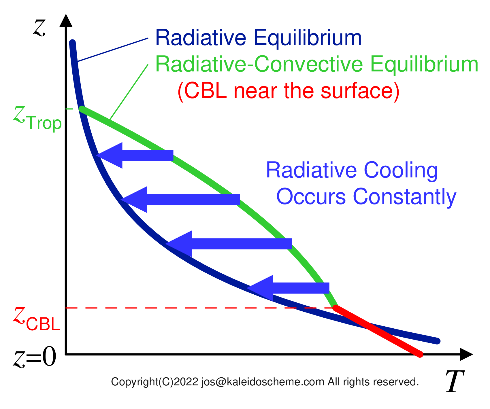
Figure 2. .
Schematic diagram for the vertical temperature profiles in radiative equilibrium (shown with the dark-blue-colored line) and radiative-convective equilibrium (the green-colored line) of the atmosphere. The horizontal and vertical axes represent temperature and altitude, respectively. If the Earth's atmosphere is dominated only by solar and planetary radiation, the temperature should have a radiatively equilibrated profile. However, as the vertical gradient of the temperature profile in radiative equilibrium near the surface becomes steep and dynamically unstable, convection occurs in the troposphere as cumulus (deep convection) and CBL (shallow convection, the red-colored line) to maintain the troposphere in radiative-convective equilibrium. The symbols zTrop and zCBL on the vertical axis show the tropopause and the top of CBL, respectively. The temperature at radiative-convective equilibrium is kept generally higher than that at radiative equilibrium in most of the troposphere, except for the range of CBL that forms near the surface. That is why the radiative-convective equilibrium atmosphere will be subject to radiative cooling constantly, until it settles down into the radiatively equilibrated state (as shown with blue arrows). Note that this radiative cooling is not originated in excessive heating of the atmosphere over the radiative-convective equilibrium due to dynamical forcing from the cumulus motion. The troposphere needs to involve steady radiative cooling, by just being maintained in radiative-convective equilibrium.
On the other hand, if we look at the tropospheric atmosphere outside the cumulus, the atmosphere is constantly undergoing radiative cooling as shown in Fig. 2. The interpretation, that radiative cooling occurs because the air blowing out from the top of the cumulus pushes down and heats adiabatically the atmosphere around the cumulus, is incorrect. Since the tropospheric atmosphere is maintained in a state of radiative-convective equilibrium, which is out of radiative equilibrium, radiative cooling will continue to occur without any forcing until the troposphere settles into radiative equilibrium. Radiative cooling continues to occur because the temperature of the radiative-convective equilibrium atmosphere is higher than that of the radiative equilibrium atmosphere at most points in the troposphere. In reality, however, the tropospheric atmosphere is maintained at the radiative-convective equilibrium temperature and does not cool down to the radiative equilibrium temperature by radiative cooling. What kind of motion of the atmosphere can maintain such a thermal equilibrium state?
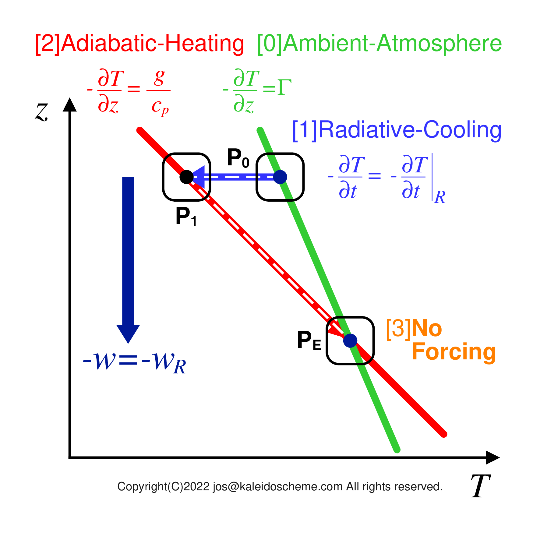
Figure 3. .
Horizontal and vertical axes are temperature and altitude, respectively. The round-squares (with points at the centers) show an air parcel at the initial P0 and subsequent states P1 and PE after a unit time, respectively. Assuming that the ambient atmosphere is maintained at the radiatively-convectively equilibrated temperature with a temperature lapse rate Γ (the green-colored line [0]), consider an air parcel at an arbitrary point P0 in the troposphere. As shown in Fig. 2., even if the air parcel is not forced by the cumulus motion, it undergoes radiative cooling -δT/δt|R, its temperature decreases, and it transitions to state P1 (the blue-colored arrow with white broken pin-line [1]). In state P1, the temperature of the air parcel is lower than the temperature of the ambient atmosphere (line [0]), and the air parcel sinks with a subsidence velocity -w due to negative buoyancy. As the air parcel sinks, it undergoes adiabatic heating at a rate of (g/cp)(-w) (the red-colored arrow with white broken pin-line [2]). When the subsidence velocity -w is equal to a certain equilibrium velocity -wR, the sinking point reaches state PE, where the temperature of the air parcel and the temperature of the ambient atmosphere coincide. In state PE, the air parcel is not forced by the ambient atmosphere (shown as [3]). Nor is the equilibrium state of the ambient atmosphere disturbed by the subsidence of the air parcel.First, for the sake of explanation, assume that the tropospheric atmosphere is maintained at radiative-convective equilibrium temperature by some mechanism.
[NOTE]
In fact, this mechanism is what RDC is, which will be described below. But for now, please accept it as "some mechanism". Since we are talking about the equilibrium state between the mean components of the atmosphere, it is sufficient to establish a consistent relationship, not a causal one as in dynamics. In the RDC scheme, the dynamics is calculated separately from the RDC relationship, and the dynamics treats disturbant components of the atmosphere that are displaced from the mean components. Therefore, the RDC scheme is guaranteed to represent even the transition of equilibrium states due to dynamical forcing.When an air parcel at a certain height in the troposphere is subjected to radiative cooling, its temperature decreases and it sinks due to negative (vertically downward) buoyancy. As the air parcel sinks, adiabatic heating will cause the temperature of the air parcel to increase. If the sinking air parcel continues to sink at a rate such that its temperature is always the same as the temperature of the ambient atmosphere, it will not feel any forcing from its surroundings, and its sinking motion will not disturb the thermal equilibrium in the ambient atmosphere. For the sake of explanation, we have assumed at the beginning that the tropospheric atmosphere is maintained at radiative-convective equilibrium temperature. But if all the air parcels in the troposphere perform this kind of motion, the entire troposphere can be maintained at the radiative-convective equilibrium.
[NOTE]
It has long been known that such subsidence flows are generally observed outside of cumulus clouds. No one would question this fact.The formulation of this local thermodynamical balance is the first basic equation used in the RDC parameterization. Figure 3. shows the local thermodynamical balance for an arbitrary air parcel in the troposphere. Given the radiative cooling rate -δT/δt|R on an arbitrary air parcel, it is possible to calculate the corresponding subsidence velocity -wR of the air parcel. For the sake of consistency with other equations, wR is assumed to be the vertical upward velocity (taking a negative value). Using the gravity acceleration g and the specific heat of the atmosphere at constant pressure cp, the dry adiabatic lapse rate can be written as g/cp. As the air parcel sinks, it is heated by adiabatic heating at a rate (g/cp)(-wR). The temperature of the ambient atmosphere, which has an temperature lapse rate Γ=-δT/δz, also increases at a rate of Γ (-wR).
Therefore, if the rate at which the air parcel is excessively heated by the sinking motion over the ambient atmosphere is balanced by the radiative cooling rate applied to the air parcel, we can write the relationship \begin{eqnarray} {\left( \frac{g}{{c}_{p}} - \Gamma \right)} \left(-{w}_{R}\right) = - {\left. \frac{\partial {T}}{\partial t} \right|}_{R} \label{balance}. \end{eqnarray}
[NOTE]
The right-hand side of Eq. (\ref{balance}) is the radiative cooling rate. This is because radiative cooling is generally the primary and only heat sink in clear sky regions. If, under special circumstances, a heat source/sink other than radiative cooling is present, we can place the term for that heat source/sink on the right-hand side. Thus, RDC can be easily generalized to include thermal processes other than radiative cooling in situations where dynamic circulation is difficult to achieve. In this case, the name RDC should be replaced with TDC, Thermodynamically Driven Circulation.From this, the thermodynamically balanced vertical velocity wR can be obtained as \begin{eqnarray} {w}_{R} = {\left( \frac{g}{{c}_{p}} - \Gamma \right)}^{-1} {\left. \frac{\partial {T}}{\partial t} \right|}_{R} \label{wR}. \end{eqnarray}
As long as the air parcel continues to move at the vertical velocity wR (typically a subsidence velocity with a negative value) described by Eq. \eqref{wR}, it is not subject to any forcing, including buoyancy. At the same time, the current radiative-convective equilibrium state of the ambient atmosphere is maintained when the air parcel has the vertical velocity wR.
[NOTE]
Let's estimate the value for the equilibrium vertical velocity wR, using typical values for the Earth's atmosphere. The physical constants for the gravity acceleration and the specific heat for dry air are given as g=9.8 m s-2 and cp=7R/2=1004.675 J K-1, where R = 2.8705 × 10² J K−1 is the gas constant, respectively. And let's assume that the typical values of the temperature lapse rate and the radiative cooling rate are Γ=6.5 K km-1=6.5 × 10⁻³ K m-1 and -δT/δt|R=2 K day-1= 2.31 × 10⁻⁵ K s-1, respectively. Then the typical value of the radiatively driven vertical velocity wR in the MKS unit system can be estimated from Eq. (\ref{wR}) as \begin{eqnarray} {w}_{R} & = & {\left( \frac{9.8}{1004.675} - 6.5 \times {10}^{-3} \right)}^{-1} \times \left(- 2.31 \times {10}^{-5}\right) \nonumber \\ & \sim & -7.1 \times {10}^{-3}. \nonumber \end{eqnarray} The negative value -7.1 mm s-1 for the radiatively driven vertical velocity wR is consistent with the subsidence velocity observed in the real atmosphere of about 1 cm s-1. (We may have written somewhere that the observed subsidence rate is about 1mm s-1, but 1cm s-1 is more appropriate.) This agreement suggests that the radiatively driven subsidence wR is actually realized in the real atmosphere.[NOTE]
In Fig. 3, we have assumed that first radiative cooling, then negative buoyancy, and finally adiabatic heating act on the air parcel to determine the subsidence velocity -wR of the air parcel in that order. And therefore, we can call the subsidence velocity -wR as "radiatively driven subsidence velocity". In reality, however, the order in which the physical processes act is irrelevant. Since all of these physical processes occur in an equilibrium atmosphere, they need only to be consistent with each other. In fact, we will consider below the cases where the subsidence velocity -w does not have the equilibrium value -wR, but even in such cases, the air parcel will eventually adjust to have the equilibrium subsidence velocity -wR.However, is it possible for the velocity w of each air parcel to have the equilibrium value wR so conveniently? In fact, it is inevitable that w takes only the value wR and cannot take any other value. This will be explained below.
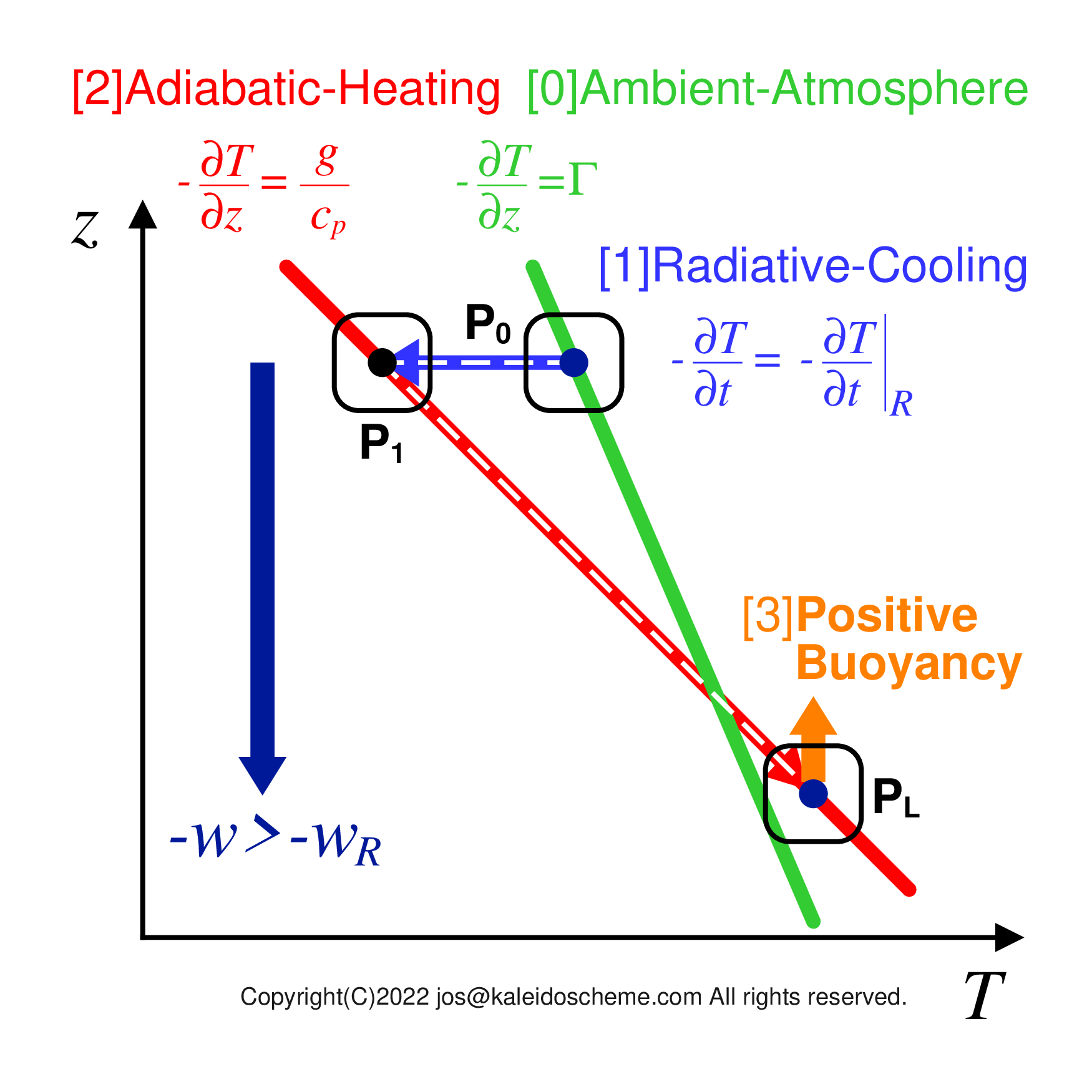
Figure 4. .
Case of a larger subsidence velocity -w >-wR. When the air parcel sinks, the adiabatic heating becomes larger than the radiative cooling to make the air parcel warmer than the ambient atmosphere (as shown with PL). The air parcel is buoyed and its subsidence velocity is forced back to -wR. Thus, even if such subsidence velocity occurs, it is immediately corrected to -wR shown in Fig. 3. Note that the radiative cooling is independent of the subsidence velocity -w. (See Fig. 5 for the opposite case.)If, for example, a given air parcel has a subsidence velocity -w that is larger than -wR (-w > -wR as shown in Fig. 4. NOTE: We are comparing the absolute values of the negative velocities w and wR here), it will be subjected to excess adiabatic heating and thus become warmer than the ambient atmosphere, and will be dynamically forced to have a subsidence velocity -wR by the upward (positive) buoyancy, which is a restoring force.
[NOTE]
Although RDC theory considers the mean atmospheric field, it may be easier to intuitively understand how this restoring force works in the real atmosphere. If the excess downward velocity is small enough to lower the position of the air parcel slightly below its equilibrium position, this restoring force will quietly return the air parcel to its proper equilibrium position. However, if the downward velocity is so great that the air parcel is pushed down a finite distance past its equilibrium position, a disturbance is added to the atmosphere, and this restoring force acts as the actual restoring force in a wave phenomenon. This is the typical situation for internal gravity wave generation, which is actually observed in real and model atmospheres.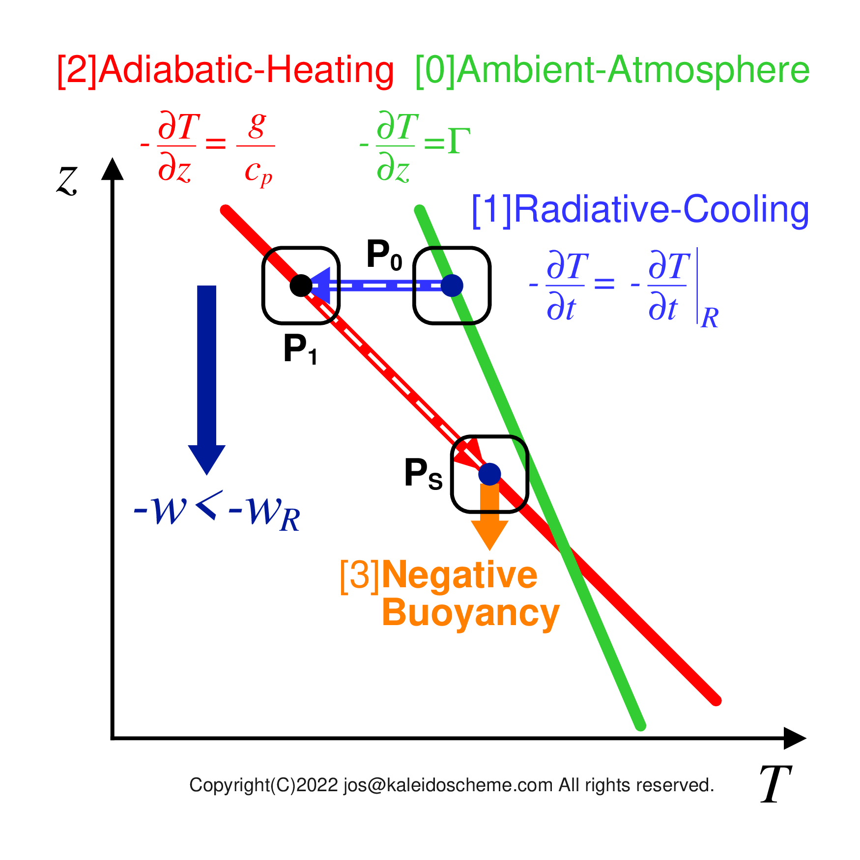
Figure 5. .
Case of a smaller subsidence velocity -w <-wR. When the air parcel sinks, the adiabatic heating becomes smaller than the radiative cooling to make the air parcel cooler than the ambient atmosphere (as shown with PS). The air parcel is negatively buoyed and its subsidence velocity is forced back to -wR. Thus, even if such subsidence velocity occurs, it is immediately corrected to -wR shown in Fig. 3. Note that the radiative cooling is independent of the subsidence velocity -w. (See Fig. 4 for the opposite case.)Conversely, if the subsidence velocity -w of the air parcel is less than -wR (-w < -wR as shown in Fig. 5.), the air parcel cannot obtain sufficient adiabatic heating to compensate for the radiative cooling and becomes cooler than the ambient atmosphere, and is dynamically forced to have a subsidence velocity -wR due to the downward (negative) buoyancy, which is again a restoring force.
[NOTE]
Here again, as shown in the Note for Fig. 4, it is intuitively easier to understand how the restoring force works rather in the real atmosphere. If the lack of downward velocity is sufficiently small, the air parcel is quietly returned to its equilibrium position by this restoring force. However, if the deficiency in downward velocity is large, a finite disturbance is added to the atmosphere, and this restoring force actually functions as a restoring force in internal gravity waves.
Here the subsidence velocity wR was derived using the separate steps from [0] to [3] to emphasize the causal relationship. Taking the time step infinitesimal, however, radiative cooling and subsidence motion are regarded to occur simultaneously and continuously in the local thermodynamical balance. So the air parcel is actually restricted to move along the ambient atmosphere line [0] rather than through a point such as P1, which is outside of the line [0]. As long as radiative cooling continues, this subsidence velocity -wR remains steady. Without this subsidence velocity -wR, the thermodynamical equilibrium in the atmosphere would not be maintained.
As shown above, any air parcel in the troposphere in a state of radiative-convective equilibrium will always be dynamically bound to have a vertical motion (sinking motion) of -w = -wR. If all the air parcels in the troposphere move with their own subsidence velocities -w = -wR, respectively, the entire troposphere can maintain the radiatively-convectively equilibrated state. The sinking motion is not only steady but also stable. If an air parcel is in the same vertical motion as the ambient atmosphere, it does not feel any forcing, but if it tries to move even slightly differently, it is restored back to the same motion -w = -wR as the ambient atmosphere with a strong binding force. This is an extremely strict constraint. It is especially worth to comment that the vertical motion of the air parcel shown here does not require any forcing from the dynamical flow associated with cumulus motion, including dynamical detrainment or anything like that. The subsidence motion occurs in the equilibrium atmosphere.
[NOTE]
Since the issue here is buoyancy, it is more rigorous to use a virtual temperature Tv that takes into account the effect of the partial pressure of water vapor \begin{eqnarray} {T}_{v} = \left( 1 + 0.608 {q}_{v} \right) T \label{Tv}, \end{eqnarray} where qv is water vapor mixing ratio, instead of temperature T. However, replacing temperature T with virtual temperature Tv does not change the essential argument. It is because the contribution from the second term is very small, and because the water vapor mixing ratio qv in the air parcel does not change in the subsiding motion. For the sake of simplicity, the discussion is shown here based on temperature T. For a more rigorous discussion, replace the temperatures T with the corresponding virtual temperatures Tv.Note that the right-hand side of Eq. \eqref{wR} is a product of two factors: the inverse of the difference between the different temperature lapse rates (g/cp-Γ)-1 and the radiative heating rate δT/δt|R. In a clear, cloudless sky, neither factor varies rapidly in the vertical direction, and therefore the thermodynamically balanced vertical velocity wR given by Eq. \eqref{wR} does not vary rapidly in the vertical direction either.
Equation \eqref{wR} multiplied by the atmospheric density ρ yields the upward vertical mass flux (typically a subsidence mass flux with a negative value) \begin{eqnarray} \rho {w}_{R} = \rho {\left( \frac{g}{{c}_{p}} - \Gamma \right)}^{-1} {\left. \frac{\partial {T}}{\partial t} \right|}_{R} \label{Fmz}. \end{eqnarray}
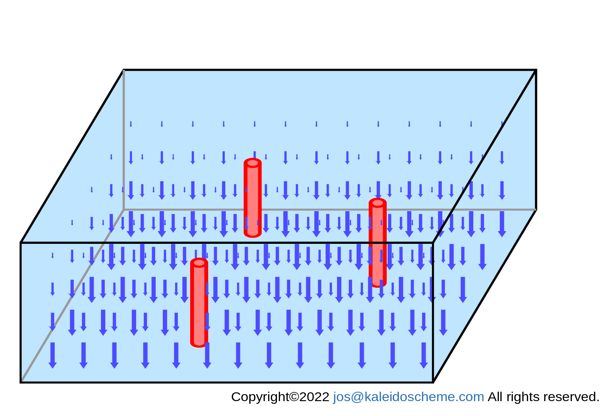
Figure 6. .
Schematic representation of the subsidence mass fluxes ρ wR (Eq. \eqref{Fmz}) thermodynamically balanced with radiative cooling in the computational area. The subsidence mass flux is shown as a downward-pointing blue arrow at each computational grid-point in the atmosphere. The subsidence mass flux has small values in the upper layers and large values in the lower layers, resulting in a mass divergence field throughout the troposphere, which alone cannot sustain a flow field, because a vacuum is created everywhere in the troposphere.
If there is no object with strong optical properties in the troposphere, this subsidence mass flux (given by Eq. \eqref{Fmz}) is essentially a divergent field, as shown in Fig. 6.
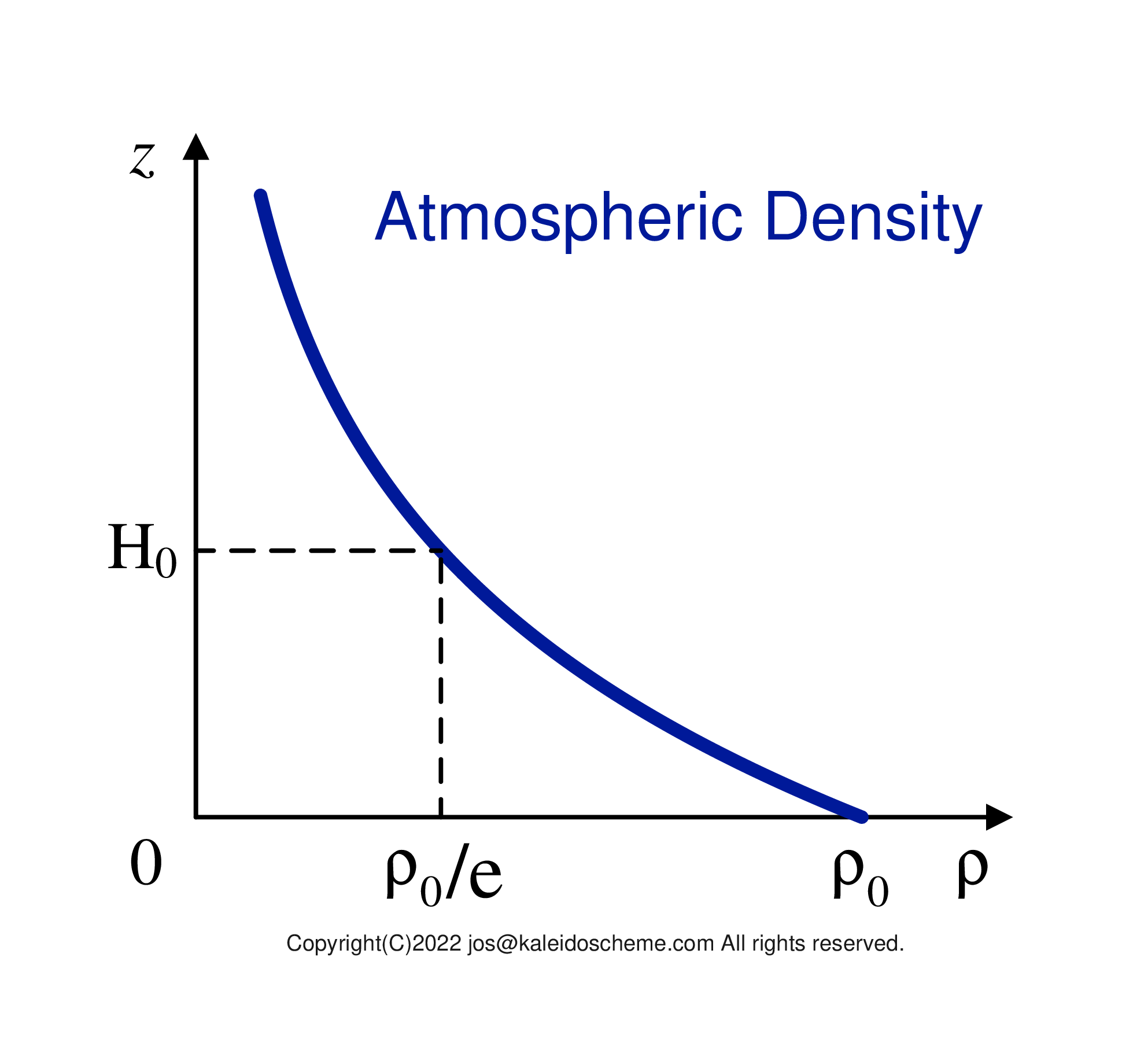
Figure 7. .
Schematic diagram for vertical profile of the atmospheric density ρ, with the value ρ0 near the surface. The vertical gradient is exponentially steep with respect to the height z. The scale-height H0 is usually taken between several kilometers and ten kilometers.
This is because the vertical velocity wR given by Eq. \eqref{wR} does not vary rapidly in the vertical direction, while the atmospheric density shown in Fig. 7 \begin{eqnarray} \rho \left(z\right) = {\rho}_{0} \exp \left( -\frac{z}{{H}_{0}} \right) \label{rho}, \end{eqnarray} which is multiplied by the vertical velocity wR in Eq. \eqref{Fmz}, has a very large exponential slope with respect to height z. Here, H0 is the scale-height of the atmosphere.
Taking the z-derivative of both sides of Eq. \eqref{Fmz}, the divergence of the vertical mass flux can be written as \begin{eqnarray} \frac{\partial}{\partial z} \left( \rho {w}_{R} \right) = \frac{\partial}{\partial z} \left[ \rho {\left( \frac{g}{{c}_{p}} - \Gamma \right)}^{-1} {\left. \frac{\partial {T}}{\partial t} \right|}_{R} \right] \label{diver}. \end{eqnarray}
[NOTE]
In general, in clear sky atmosphere, when considering the vertical gradient of the vertical mass flux (Eq. \eqref{diver}), contribution from the atmospheric density ρ (Eq. \eqref{rho}) is dominant relative to that from the rest part throughout the troposphere, no matter what radiation calculation scheme is used. Therefore, the mass divergence (Eq. \eqref{diver}) due to the subsidence mass flux ρwR (Eq. \eqref{Fmz}) is always positive, independent of the details of the radiative calculation scheme.[NOTE]
In regions where there are objects with strong optical properties in the atmosphere, such as clouds, the vertical gradient of the radiative cooling rate -δT/δt|R may locally be larger than the vertical gradient of the atmospheric density ρ (given by Eq. \eqref{rho}) in Eq. \eqref{diver}. In this case, the effect of the radiative cooling distribution may modify the uniform mass divergence field in the troposphere. As you can imagine from the following explanation, special outflows and inflows in horizontal directions can occur in such a field, which can lead to interesting phenomena (e.g., Iwasa et al. 2012). -
Continuity of the Atmosphere
Since the vertical mass flux ρwR (Eq. \eqref{Fmz}) has a mass divergence (Eq. \eqref{diver}) throughout the troposphere, a vacuum is created everywhere by the vertical flow alone. To compensate for this, a horizontal mass flux (ρuR, ρvR) must be induced (sucked out) in the atmosphere. The formulation of this process is based on the equation of continuity \begin{eqnarray} \frac{\partial}{\partial x} \left(\rho {u}_{R}\right) +\frac{\partial}{\partial y} \left(\rho {v}_{R}\right) +\frac{\partial}{\partial z} \left(\rho {w}_{R}\right) = 0 % \left(z\right) = {\rho}_{0} \exp \left( % -\frac{z}{{H}_{0}} % \right) \label{continuity}, \end{eqnarray} which specifies the mass continuity in the three-dimensional atmosphere. This is the second basic equation used for RDC parameterization.
Substituting Eq. \eqref{diver} into Eq. \eqref{continuity} yields \begin{eqnarray} \frac{\partial}{\partial x} \left(\rho {u}_{R}\right) +\frac{\partial}{\partial y} \left(\rho {v}_{R}\right) = - \frac{\partial}{\partial z} \left[ \rho {\left( \frac{g}{{c}_{p}} - \Gamma \right)}^{-1} {\left. \frac{\partial {T}}{\partial t} \right|}_{R} \right] \label{rdc}. \end{eqnarray} Equation \eqref{rdc} is the final form of the equation that expresses the basic principle of RDC in a three-dimensional atmosphere. Note that the value of the right-hand side of Eq. \eqref{rdc} is already known, because the density ρ, temperature lapse rate Γ, and radiative cooling rate -δT/δt|R are obtained from the atmospheric model. -
Flow Field with No Vertical Vortices
At this point, Eq. \eqref{rdc} alone is one equation short, since the unknown variables are the two components of the two-dimensional horizontal mass flux, ρuR and ρvR. As we are describing the simplest principle for applying RDC to parameterization, we will give, for example, the condition for a flow field with zero rotation in the z direction everywhere
\begin{eqnarray} \frac{\partial }{\partial x} \left(\rho {v}_{R}\right) -\frac{\partial}{\partial y} \left(\rho {u}_{R}\right) = 0 \label{rot0}. \end{eqnarray}Equation \eqref{rot0} is used here as another counterpart to Eq. \eqref{rdc}. Neither equation includes z-dependence. Therefore, by solving the simultaneous differential equations, Eqs. \eqref{rdc} and \eqref{rot0}, under appropriate boundary conditions on the horizontal plane at each altitude, we can obtain the two-dimensional horizontal mass flux field (ρuR, ρvR).
If you want to take the Coriolis force into account for RDC, you can replace zero on the right-hand side of Eq. \eqref{rot0} by a function expressing the contribution from the Coriolis force. Even in that case, the Coriolis force will depend at most only on latitude y, so the physical argument here does not require any essential modification.
[NOTE]
The low-latitude regions of the tropics and subtropics, which have the greatest influence on the climatological radiation budget because they cover the largest area of the Earth, are considered to be the regions where the RDC is the most efficient transport process due to the low Colioris force and the low influence of mid- and high-latitude disturbances. It is in these low-latitude regions that the assumption of no vertical vorticity is justified. -
Boundary Conditions
The boundary of the supplying source domain is a free boundary. That is, it only allows as much runoff (or inflow) to pass through as required by the surrounding atmosphere.
[NOTE]
However, if the atmospheric model explicitly calculates the vertical mass flux within the supplying source domain, and only if that vertical mass flux is not sufficient to provide air mass for the "FULL" RDC outflow given by Eq. (\ref{rdc}), then the RDC outflow should be consistently limited according to the vertical mass flux within the supplying source domain, as discussed below.For the box-shaped computational region as shown in the figures, if periodic boundary conditions are given for the physical properties φ (such as the velocities and physical values) at the boundaries, say, x=0 with x=xB, and y=0 with y=yB, of the computational region as \begin{eqnarray} \left\{ \begin{array}{ll} \phi \left({x}_{\rm{B}},y,z\right) & = & \phi \left(0,y,z\right) \\ \phi \left(x,{y}_{\rm{B}},z\right) & = & \phi \left(x,0,z\right) \end{array} \right. \label{cyclic4phi}, \end{eqnarray} the same periodic boundary conditions apply to the horizontal mass fluxes ρuR(x,y) and ρvR(x,y) as \begin{eqnarray} \left\{ \begin{array}{ll} \rho {u}_{R} \left({x}_{\rm{B}},y\right) & = & \rho {u}_{R} \left(0,y\right)\\ \rho {u}_{R} \left(x,{y}_{\rm{B}}\right) & = & \rho {u}_{R} \left(x,0\right)\\ \\ \rho {v}_{R} \left({x}_{\rm{B}},y\right) & = & \rho {v}_{R} \left(0,y\right)\\ \rho {v}_{R} \left(x,{y}_{\rm{B}}\right) & = & \rho {v}_{R} \left(x,0\right) \end{array} \right. \label{cyclic4u} \end{eqnarray} at each altitude z. The same periodic boundary conditions can be applied to the global computational region.
If the entire computational region is presegmented into small compartments (of arbitrary shapes) based on the radiative properties of the atmosphere, a condition can be applied that the horizontal mass flux does not penetrate the boundaries between the compartments at any point on the boundary lines dividing the compartments. This means that the horizontal mass flux has no component normal to the boundary, i.e., the inner product of the horizontal mass flux (ρuR, ρvR) and the normal vector (nx, ny) of the boundary line is zero \begin{eqnarray} \rho {u}_{R} {n}_{x} + \rho {v}_{R} {n}_{y} = 0 \label{noPenetrate}. \end{eqnarray}
-
Velocity Potential and Poisson Equation
Since the physical discussion is complete up to this point, solving numerically is a technical problem. As an example, we assume a vorticity-free flow (Eq. \eqref{rot0}) and reduce the number of unknown variables to one to make it easier to deal with in the model.
Vorticity-free flow (Eq. \eqref{rot0}) is automatically realized by introducing a velocity potential Φ(x,y) satisfying \begin{equation} \left\{ \begin{array}{ll} \rho {u}_{R} & = - \frac{\displaystyle \partial \Phi}{\displaystyle \partial x} \\ \rho {v}_{R} & = - \frac{\displaystyle \partial \Phi}{\displaystyle \partial y} \end{array} \right. \label{eq:potential}. \end{equation}
[NOTE]
The name "velocity potential" simply follows the conventions of mathematical physics. In this case the velocity is density weighted, so as you can see it should really be called here "mass flux potential".Substituting Eq. \eqref{eq:potential} into Eq. \eqref{rdc} \begin{eqnarray} \frac{\partial}{\partial x} \left( - \frac{\displaystyle \partial \Phi}{\displaystyle \partial x} \right) +\frac{\partial}{\partial y} \left( - \frac{\displaystyle \partial \Phi}{\displaystyle \partial y} \right) = - \frac{\partial}{\partial z} \left[ \rho {\left( \frac{g}{{c}_{p}} - \Gamma \right)}^{-1} {\left. \frac{\partial {T}}{\partial t} \right|}_{R} \right] \end{eqnarray} yields a Poisson equation \begin{eqnarray} \frac{{\partial}^{2} \Phi}{\partial {x}^{2}} + \frac{{\partial}^{2} \Phi}{\partial {y}^{2}} = \frac{\partial}{\partial z} \left[ \rho {\left( \frac{g}{{c}_{p}} - \Gamma \right)}^{-1} {\left. \frac{\partial {T}}{\partial t} \right|}_{R} \right] \label{poisson}. \end{eqnarray}
Boundary conditions can also be rewritten for Φ. In the case of the periodic boundary condition Eq. \eqref{cyclic4u}, a similar condition \begin{eqnarray} \left\{ \begin{array}{ll} \Phi \left({x}_{\rm{B}},y\right) & = & \Phi \left(0,y\right), \\ \Phi \left(x,{y}_{\rm{B}}\right) & = & \Phi \left(x,0\right) \end{array} \right. \label{cb4Phi} \end{eqnarray} can be used.
When the calculation region is presegmented into compartments, substituting Eq.\eqref{eq:potential} into Eq. \eqref{noPenetrate} provides the boundary condition on the dividing boundary lines as \begin{eqnarray} % \left(- \frac{\displaystyle \partial \Phi}{\displaystyle \partial x}\right) % {n}_{x} % + % \left(- \frac{\displaystyle \partial \Phi}{\displaystyle \partial y}\right) % {n}_{y} = 0,\nonumber %\\ {n}_{x} \frac{\displaystyle \partial \Phi}{\displaystyle \partial x} + {n}_{y} \frac{\displaystyle \partial \Phi}{\displaystyle \partial y} = 0 \label{noPenetrate4Phi}. \end{eqnarray}
Thus, in the case of vorticity-free flow, the calculation of the RDC parameterization ultimately boils down to solving the Poisson equation Eq. \eqref{poisson} for the scalar variable velocity potential Φ(x,y) in the horizontal two-dimensional plane at each altitude, under boundary condition Eq. \eqref{cb4Phi}, \eqref{noPenetrate4Phi}, or something appropriate. As you see, this is a very ordinary two-dimensional Poisson-type boundary value problem. Therefore, it can be solved numerically using a general-purpose boundary value problem solver package without writing any special program. Once Φ is obtained by correctly solving this boundary value problem, a horizontal mass flux (ρuR,ρvR), consistent with the subsidence mass flux ρwR given in Eq. \eqref{Fmz}, can be obtained from Eq. \eqref{eq:potential}.
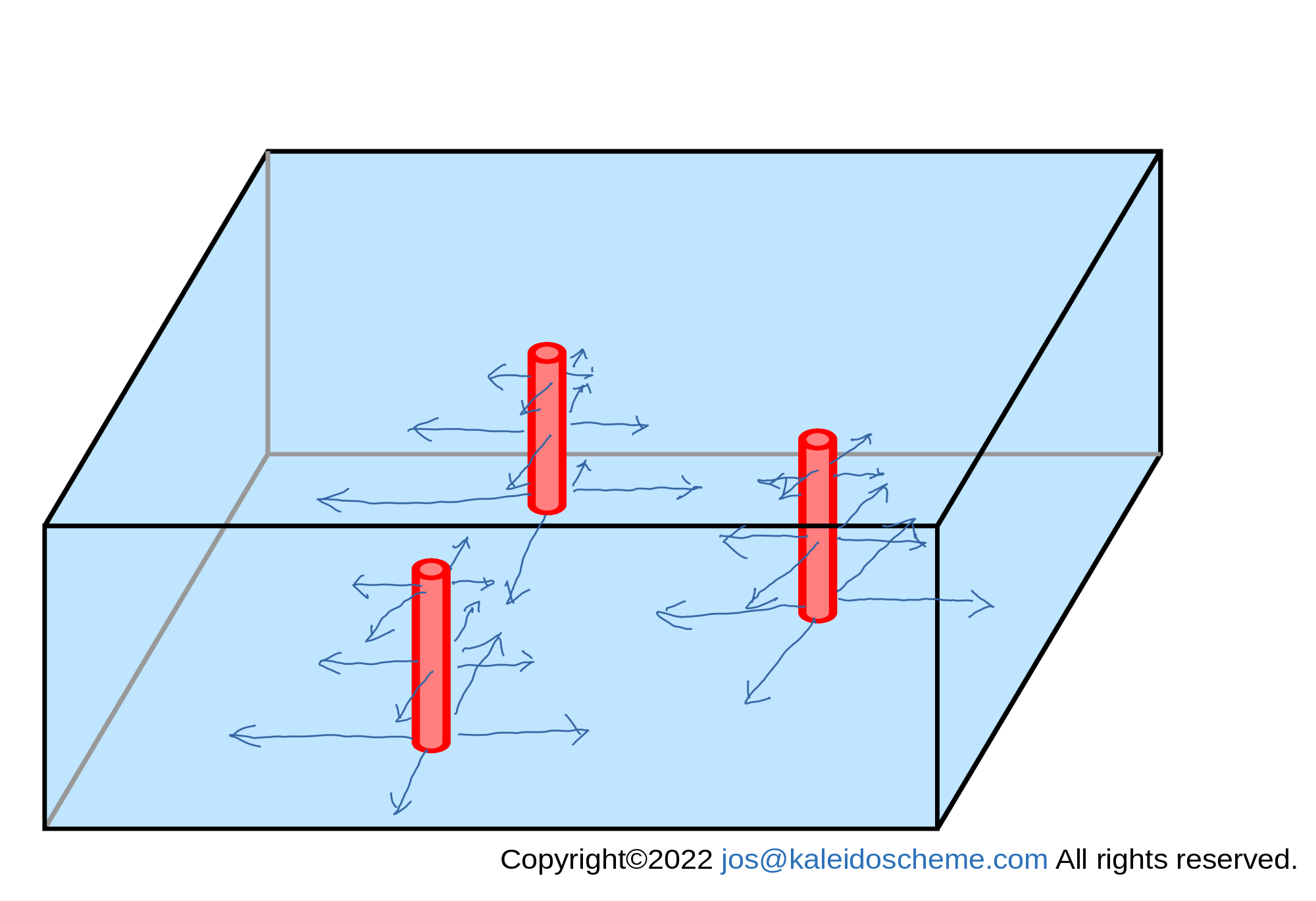
Figure 8. .
Convergent horizontal mass fluxes induced outward from the supplying source (cumulus) domains to compensate for the divergence of the subsidence mass fluxes shown in Fig. 6.: the outgoing horizontal mass flux has a larger value closer to the supplying source domain and a smaller value away from it. Although the figure shows only a limited number of outflows, outflows actually occur in all argument directions around the supplying source domain.
Figure 8. shows a conceptual diagram of the horizontal mass fluxes (ρuR,ρvR). As described in Fig. 6., the subsidence mass fluxes ρwR are generally mass divergent, so the compensating horizontal mass fluxes (ρuR,ρvR) shown in Fig. 8 are mass convergent and are induced from the supplying source domains.
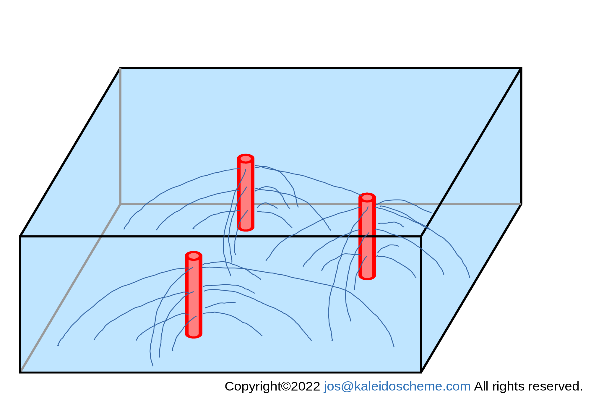
Figure 9. .
Conceptual streamlines of RDC around the supplying source domains, which are formed by the divergent subsidence mass fluxes and the convergent horizontal mass fluxes shown in Figs. 6 and 8, respectively. Although only a limited number of streamlines are shown in the figure, outflows actually occur in all argument directions around the supplying source domain.
The three-dimensional mass flux ρuR = (ρuR,ρvR,ρwR) produced by the RDC is shown conceptually in Fig. 9. At every altitude in the troposphere, there is an outflow from the supplying source domain to the outside.
The mass flux ρuR = (ρuR,ρvR,ρwR) obtained by the above procedure is divided by the atmospheric density ρ to give the RDC velocity uR = (uR,vR,wR). Adding the velocity field uR obtained by RDC parameterization to the velocity field uL* obtained by explicitly solving the equation of motion (after removing the effect of radiative cooling consumed by RDC; but perhaps this removal is needed only for the equation predicting temperature) yields the actual velocity field u = uL*+uR in the atmospheric model.
-
Flows in the Convective Boundary Layer (CBL)
The RDC mechanism described above operates within the troposphere, except for the CBL generated near the surface, which is dominated by convective rather than radiative processes. Thus, the RDC has no ACTIVE flow in the CBL. However, air flowing out of the cumulus flank must return to the cumulus root within the CBL to satisfy mass continuity. Therefore, within the CBL, it is acceptable to assume that the vertically-uniform PASSIVE horizontal mass flux is directed toward the cumulus so as to maintain the mass balance throughout the troposphere. By adding such a consistent flow within the CBL, the RDC is able to represent the flow in the model as a complete circulation, closing the streamlines. Of course, if the model can explicitly handle convective motion in the CBL, the resulting dynamical flow can be added to the passive RDC flow. -
RDC as a Universal Mechanism
Since RDC is a universal mechanism, independent of latitude or region, it is assumed to operate at mid and high latitudes as well as at low latitudes. However, in such regions, the supplying source domain is not necessarily a single cumulus cloud, and it may be necessary to assume an organized mass of disturbances. At mid and high latitudes, in addition, mesoscale and synoptic scale disturbances may be larger than RDC and RDC may be masked by the noise of these disturbances. To extract the RDC component, it may be necessary to apply some sort of filter to remove the noise, rather than a simple time average. Alternatively, if strong dynamical disturbances are dominant and responsible enough for mass/heat/water vapor transport at mid and high latitudes, there is no need to consider the ignorable RDC in this region.
Many well-known phenomena can be reinterpreted to be based on RDC. For example, the Hadley circulation has been mainly treated as a forced circulation due to equatorial cumulus convection, but it is more natural to consider it as an RDC due to radiative cooling in the extra-equatorial region.
Dr. Naohiko Hirasawa, who is one of the best understanders of RDC, suggested in our discussion twenty years ago that the Katabatic winds seen at the Antarctic continental margin are not only due to near-surface cooling, but rather are the result of air that has cooled and sunk throughout the troposphere and has no place to go near the surface and is blown out to the continental margin. This explains much stronger Katabatic winds.
And although this is our personal opinion and needs to be verified, we believe that many "remote effects" based on the dynamical forcing of cumulus convection should be rejected and, rather, reinterpreted as field-dependent phenomena through large-scale RDC mechanism.
Furthermore, rewriting the differentiable term on the right-hand side of Eq. (\ref{poisson}), which describes the effects of radiative cooling and excess adiabatic heating, to incorporate other processes, such as chemical reactions, nuclear fission/fusion, magnetohydrodynamic processes, and possibly biological processes, may extend its application to explain flow phenomena within regions of the Earth's atmosphere beyond the troposphere, as well as within the “atmospheres” of other planets and stars. This approach may also be applicable to “flow” in liquid and solid phases, not just the gas phase. All of these will be variants of the RDC scheme, which could be called the "X"DC scheme, because those flows may driven by other physical processes than Radiative cooling.
-
Applying Cases
[case-A]
With a large computational region and a time interval ΔtR for FR calculations long enough, there are likely sufficient supplying source domains for outflows to compensate the mass divergence within the subsidence region. In such cases, the RDC parameterization described above can be perfectly applied.[case-B]
In the most extreme case, when the presegmented compartments are small and the time interval ΔtR is short, for example, there may be no supplying source domains at all in some computational compartments. In such cases, RDC parameterization cannot be applied. The atmosphere cannot subside due to the lack of horizontal compensating flow, and will lower its temperature due to radiative cooling. However, this is a physically consistent phenomenon because the atmosphere becomes dynamically unstable if this situation persists, causing the formation of new cumulus clouds that subsequently become supplying source domains. That is to say, it is correct not to apply RDC parameterization when there is no supplying source domains.[case-C]
A problem is an intermediate case between the above two: when a supplying source domains exist, but the upward mass flux in the domain is not sufficient to compensate for all the mass divergence of the subsidence flow over the horizontal segment of possible reach of the RDC flow, the RDC parameterization needs to be partially applied. Although there are various patterns of partial application of RDC, the brief discussion in the following sections shows that only a method, that compensates for mass divergence at a uniform rate over the entire reachable region of the RDC flow, is possible. -
About Cumulus Mass Flux
As far as it is a parameterization, it cannot automatically predict everything. The same is true for the RDC cumulus parameterization. A few things in the RDC parameterization must be provided externally to ensure that the parameterization gives correct effects. First of all, we need to provide externally
-
supplying source domains and their internal physical values
except for the internal vertical mass flux
(as mentioned above).
[NOTE]
Previous versions of this document stated that vertical mass flux at the base of the cumulus cloud was required. That was incorrect. The vertical mass flux is not always required as explained here.
This is similar to other cumulus parameterizations and is omitted here. Since the vertical mass flux within cumulus clouds may be treated differently by different atmospheric models, we will consider the cases separately here.If your atmospheric model is not capable of predicting the vertical mass flux within the cumulus, you can use the expected vertical mass flux within a supplying source domain as a rough estimate for the mass flux within the corresponding cumulus domain, assuming that the full RDC is always realized around all possible cumulus clouds. In this case, there is no need to consider the horizontal region partitioning or the RDC flux constraints described below. The full RDC fluxes (and then the consistent vertical mass fluxes in the cumulus domains) can be obtained by feeding the model values as they are into a solver package for the boundary-value problem of Eq. \eqref{rdc}. The actual cumulus mass flux in the model should not be far from the reference mass flux obtained in this way. If they were significantly different, the equilibrium state of the surrounding atmosphere would be altered; a dynamical forcing (pushing air down) would be applied to heat the surrounding atmosphere when the actual cumulus mass flux is greater than the reference value, while a radiative cooling would be applied to the surrounding atmosphere when the actual cumulus mass flux is less than the reference value.
If your atmospheric model is capable of predicting the vertical mass flux in the cumulus, you will need to adjust the actual RDC to match the mass flux in the cumulus predicted by the model. First, consider the case of a very large vertical mass flux in the cumulus. Even after the full RDC outflow has occurred, there should still be some vertical mass flux remaining. In this case, the remaining vertical mass flux is used for the dynamic forcing process by the cumulus through the equations of motion in the model. This is naturally expressed in the RDC calculation procedure and requires no special treatment.
On the other hand, if the vertical mass flux in the cumulus cloud is less than that required to achieve full RDC outflow, the full RDC cannot be realized. Therefore, we need to provide externally
- a method to limit the RDC subsidence flow when the vertical mass fluxes in the supplying source domains are insufficient.
The following describes this limitation method.When the RDC subsidence velocity expressed with Eq. \eqref{wR} is perfectly realized in the model, the radiative cooling is eliminated by adiabatic heating due to the RDC subsidence flow. (If extra upward mass flux in the cumulus remains after being consumed by the RDC outflow, it will be used in the large-scale dynamics treatment.) However, such a balance may not be achieved in all cases. When there is no supplying source domain at all, it is easy to assume that there is no RDC subsidence flow at all, which is fine. (The unresolved radiative cooling is then all used in the temperature prediction equation. This radiative cooling eventually destabilizes the atmosphere dynamically and causes the next cumulus cloud to develop.) But when there are only inadequate supplying source domains, it is necessary to specify how RDC subsidence flow will be limited.
We have no experience in actually applying RDC cumulus parameterization in a 3D atmospheric model. Therefore, we have as yet no established method for such limitation, and it is left as a parameter tuning for numerical model operations. However, the RDC parameter tuning is expected to be much easier than that for dynamical detrainment, because:
- It only restricts the RDC flow, it does not add any flows.
- It is not necessary to observe the real atmosphere, but only to make the results of the RDC model close to that of the corresponding cumulus-resolving model.
An RDC diagnostic analysis on the results of a simple, small cumulus-resolving model under the same conditions, but assuming that all the RDC flows are fully realized, would provide good suggestions for parameter tuning on the RDC model.
-
supplying source domains and their internal physical values
except for the internal vertical mass flux
(as mentioned above).
-
Limitation on RDC Mass Flux and RDC-Consumed Radiative Cooling Rate
[NOTE]
If the model determines the net upward mass flux at the cumulus cloud base, then the full RDC flow may not occur when the mass flux is insufficient. Initially, we were concerned that some parameter tuning would be necessary to limit the RDC flow according to the supplied mass flux. However, the following simple idea shows that such tuning is unnecessary, and that the RDC flow can be unambiguously limited.[NOTE]
The following section with a purple background is outdated and no longer necessary. Assuming that full RDC is achieved sequentially from the lower levels of the atmosphere, it is possible to limit the RDC flow without tuning parameters, from the net upward mass flux at the cumulus cloud base provided by the model.
If you cannot see the purple-backgrounded section just below, you can skip the section by clicking this link.
==================== PURPLE-BACKGROUND: OUTDATED AND NO LONGER NECESSARY from here.
[NOTE]
The parameter tuning described here requires that the whole horizontal computational area at each altitude be partitioned into closed compartments (each of them is identified with an integer index i) within the reach of the RDCs. This is consistent with the partitioning of the whole horizontal area at a given altitude based on the distribution of the radiative cooling rate, as mentioned in 0.Partitioning the Whole Computational Area into Segmented Compartments.To ensure at a given altitude that the outflow of horizontal mass flux from the supplying source (cumulus) domain due to RDC
- does not exceed the upward mass flux in the supplying source domain
- provides a value close to that obtained in the corresponding cumulus-resolving model,
Our best approach at the moment is as follows. First, each closed compartment that RDC can reach is distinguished by an integer index i. Let's denote the name of a value in the RDC compartment i by adding the index i, for example, we denote wRi for the subsidence velocity in an RDC compartment i. Within each indexed RDC compartment, there may be one supplying source domain, multiple supplying source domains, or none.
- Within an RDC compartment i with sufficient upward mass flux in the supplying source domains, RDC is assumed to occur perfectly with the full subsidence velocity wRi given by Eq.\eqref{wR}.
- Within an RDC compartment i without a supplying source domain, no RDC is assumed to occur at all.
And,
- Within an RDC compartment i with insufficient upward mass flux in the supplying source domains,
a certain limitation is imposed on the RDC as follows.
The full subsidence velocity outside the cumulus wRi is limited to wRLi by being multiplied with a constant value L1i as \begin{eqnarray} {{{w}_{R}}_{L}}_{i} = {{L}_{\rm 1}}_{i} {{w}_{R}}_{i} \label{limitedWR}, \end{eqnarray} where the parameter constant L1i takes a value \begin{eqnarray} 0 \le {{L}_{\rm 1}}_{i} \le 1 \label{L1}. \end{eqnarray} The constant value L1i is unique to the compartment i and may differ between compartments. The limited subsidence mass flux wRLi will be used instead of wRi in the numerical model. The value L1i is a constant at a given altitude over the entire closed compartment i of possible reach of the RDC flow.
For a zeroth-order approximation, you can determine L1i as a perfect constant value that does not depend on anything (such as altitude z). This is possible when there is only one supplying source domain in the compartiment i. In this case, no parameter tuning is required, and the limiting constant value L1i can be determined under the assumption that given the cumulus mass flow in the supplying source domain at the root of the cumulus (at the top of CBL zCBL), which equals to the upward mass flux (ρw)(zCBL) multiplied with the cumulus cross section S(zCBL) at that level, is all consumed by mass outflow due to the limited RDC in the vertical range between zCBL and the cumulus height zCUM.
If you want to match the RDC results in a general case with those of the cumulus-resolving model more closely, you could make the limiting value L1i a function of altitude z and of some other physical properties \begin{eqnarray} {{L}_{\rm 1}}_{i} = {{L}_{\rm 1}}_{i} \left( z, \ldots \right) \label{L1function}, \end{eqnarray} where "..." denotes the possible physical quantities on which L1i depends. The function form of L1i will be determined from a parameter tuning so as to bring the results of the RDC model close to those of the corresponding cumulus-resolving model.
[NOTE]
Determining the limiting function \eqref{L1function} is the last remaining task in the RDC cumulus parameterization. From the standpoint of computational complexity, it is desirable to keep it as simple as possible. However, since it is only for limiting the full RDC mass flow out of the cumulus clouds which is obtained by solving the boundary problem \eqref{rdc}, the limiting function should be determined mostly from the mass flow balance only.The rest portion of radiative cooling rate after being consumed by the RDC is given as \begin{eqnarray} - {{{\left. \frac{\partial {T}}{\partial t} \right|}_{R}}_{L}}_{i} = \left( 1-{{L}_{\rm 1}}_{i} \right) \left( - {{\left. \frac{\partial {T}}{\partial t} \right|}_{R}}_{i} \right) \label{limitedRadCool}. \end{eqnarray} Note that the constant parameter L1i can be shared between Eqs. \eqref{limitedWR} and \eqref{limitedRadCool} because wRi given by Eq. \eqref{wR} is proportional to the radiative cooling rate -δT/δt|Ri. The rest portion of radiative cooling rate -δT/δt|RLi will be used in the temperature prediction equation instead of the original radiative cooling rate -δT/δt|Ri.
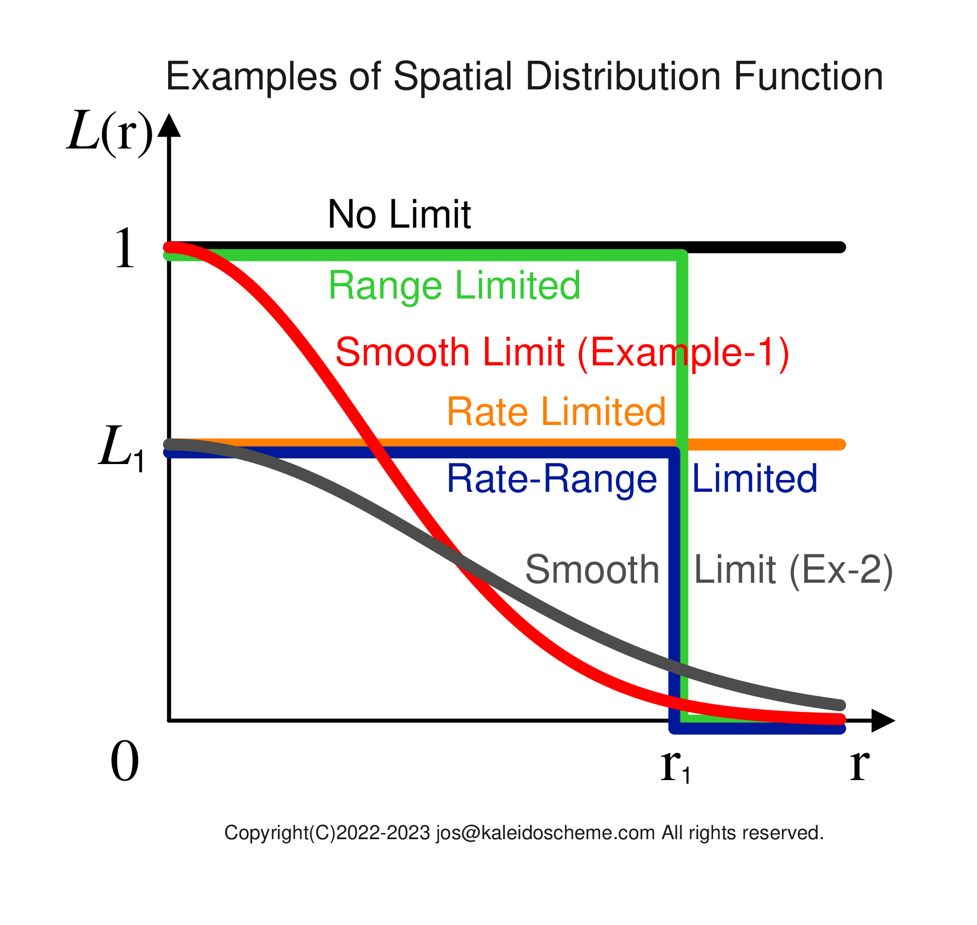
Figure 10. .
Examples of the spatial distribution function Li(r) that specifies the fraction of the limited RDC subsidence velocity wRLi (which actually occurs in the numerical model) in the overall RDC subsidence velocity wRi (which is expected by Eq. \eqref{wR} only from the radiative cooling rate -δT/δt|Ri in the atmosphere). The abscissas r shows a radial distance from the surface of the supplying source domain. The values L1i and r1i are parameters which characterize the spatial distribution functions. (Sorry, all the symbols L, L1, and r1 in the current figure lack the index i for the RDC compartment.)You may think that the limitation could be done by multiplying, not a constant L1i but some spatial distribution function Li(r) where r is a radial distance from the center of the supplying source domain, to the full RDC subsidence velocity and radiative cooling rate. In this case, the equations from \eqref{limitedWR} to \eqref{limitedRadCool} would be written in a general form as \begin{eqnarray} {{{w}_{R}}_{L}}_{i} = {L}_{i} \left( r \right) {{w}_{R}}_{i} \label{funcWR}, \end{eqnarray} where the spatial distribution function Li(r) takes a value \begin{eqnarray} 0 \le {L}_{i} \left( r \right) \le 1 \label{range4funcWR}, \end{eqnarray} and \begin{eqnarray} - {{{\left. \frac{\partial {T}}{\partial t} \right|}_{R}}_{L}}_{i} = \left( 1 - {L}_{i} \left( r \right) \right) \left( - {{\left. \frac{\partial {T}}{\partial t} \right|}_{R}}_{i} \right) \label{funcRadCool}. \end{eqnarray} Examples of the spatial distribution function are shown in Fig. 10. The possible limit functions are constant values, step functions, smooth functions of Gaussian curves, and so on.
By considering the physical meaning of RDC, however, we can choose the only available spatial distribution functions among these. RDC is a mechanism to maintain equilibrium without creating unnecessary dynamical forcing (buoyancy) in the compartment outside the cumulus. (Dynamical forcing, if needed, will be treated not by the RDC, but by the equation of motion in the atmosphere model.) Applying any function Li(r) whose value varies with the radial distance r creates a horizontal temperature difference, and therefore buoyancy, each time an RDC process occurs. This is contrary to the RDC principle. Therefore, among the spatial distribution functions shown in Fig. 10, only constant value functions with a uniform limiting rate (shown with the black and orange horizontal lines in Fig. 10) can be used in practice.
In summary, there is no need to consider the dependence of Li on horizontal distance, such as r, as incorporated in Eqs. (23)-(25). The only spatial dependence of Li is on altitude z. Of course, there remains the possibility that Li depends on other physical quantities, which should be determined by parameter tuning.
In any case, in practice, a consistent limiting method should be determined as parameter tuning by comparison with the results of the cumulus-resolving models.
[NOTE]
As time progresses, this limiting method alone may cause temperature differences between compartments (each of which is identified with the index i) at the same altitude and so undesirable buoyancy at the boundaries of the compartments. This is due to the discrete partitioning of the entire computational area in the RDC calculation procedure. However, it is expected that temperature smoothing over the compartments will probably be done automatically by the equations of motion and temperature, which are separate from the RDC calculation procedure and deal with the remaining temperature changes after they are consumed by the RDC.
==================== PURPLE-BACKGROUND: OUTDATED AND NO LONGER NECESSARY till here.
Considering that the RDC mechanism is always trying to suck out the air in the cumulus due to the mass divergence of the subsidence flow around the cumulus, it is appropriate to assume that the vertical mass flux coming up from the lower layers will be sucked out to the surroundings as soon as it becomes available. In other words, we can assume that the full RDC flow is realized starting from the lowest layer as high as possible. The RDC flow is limited only at the uppermost layer where the vertical mass flux reaches. The limited RDC flow must be distributed uniformly within the horizontal range that the flow reaches, so that local buoyancy must not be created. At the same time, the same proportion as the RDC subsidence flow being restricted should be limited in the mitigation of radiative cooling. Then, there is no longer any parameter tuning in the RDC scheme and everything can be treated as a physical calculation. It is interesting and exciting that the RDC cumulus parameterization is complete only from theory without any comparison with external results from observations and other models. Of course, we must first verify that this is indeed the case by comparing the calculations of the RDC scheme with the results of a cumulus-resolving model.
- Dynamical Detrainment flow field uD is calculated with the DD method.
-
Continuity Equation \eqref{cont4DD}:
The mass continuity of the atmosphere should be satisfied by the total velocity mass flux ρu=ρ(uL+uD).
(We doubt that this is actually satisfied. If uD is added separately to the continuity-guaranteed uL, as in the procedure shown in Fig. 1, the continuity is broken. Mass continuity in the total velocity field uL+uD, not just in the large scale flow field uL, must be considered when obtaining the large scale flow field uL.)
-
Equation of Motion \eqref{motion4DD}:
The advection velocity is the total velocity uL+uD, but it is the large field velocity uL that is predicted by the equations of motion. F on the right-hand side is the sum of the large-scale forcing terms.
-
Prediction Equation for Temperature \eqref{temp4DD}:
The right-hand side includes the first term δθ/δt|R, which is the radiative heating rate, followed by a series of heating/cooling terms due to processes other than radiation.
-
Prediction Equations for Variables Other Than Temperature \eqref{others4DD}:
Gi on the right-hand side is the sum of the creation/destruction terms for the physical quantity qi. - Radiatively Driven Circulation flow field uR is calculated with the RDC scheme.
-
Continuity Equation \eqref{cont4RDC}:
Since continuity is in principle guaranteed for the RDC velocity uR, continuity should be considered only for the large scale field velocity uL*.
-
Equation of Motion \eqref{motion4RDC}:
The total velocity u=uR +uL* is used as the advection velocity. The equation of motion predicts the large scale field velocity uL*.
-
Prediction Equation for Temperature \eqref{temp4RDC}:
Since part or all of the total radiative heating/cooling rate δθ/δt|R is consumed by the RDC, only the remaining radiative heating/cooling rate δθ/δt|R* is actually used in the temperature equations.
-
Prediction Equations for Variables Other Than Temperature \eqref{others4RDC}:
These equations would be exactly the same as for DD because they do not explicitly include a term for temperature change. - Before starting the calculation, initialize the atmospheric field. Symbols u0 and q0 on the right-hand side of the first and second expressions denote the initial fields of velocity and physical quantities of the atmosphere, respectively. In each expression, the equal sign = does not denote equality, but rather an update of the values as used in the FORTRAN language used to describe the model.
- We now have the fields of velocity u and quantities q at time t.
- Velocity field at time t+Δt can be computed using the velocity and physical quantities at time t. The flow field uL larger than the cumulus scale can be computed by solving the equation of motion FL as a time development problem. The velocity field uD contributed from the motions in the cumulus clouds is computed by a dynamical detrainment parameterization FD, which is different from the equation of motion FL for uL.
- Adding uL and uD together yields the atmospheric velocity field u=uL+uD in the model at time t+Δt.
-
Solving the respective time development equation Fq for each quantity q
yields each quantity q at time t+Δt.
(For simplicity of presentation, block 4 is placed in sequence, but it can be calculated independently and in parallel with blocks 2 and 3.) - If time t is less than the final time tMAX, then time t is updated to the new value t+Δt and the process is repeated back to block 1.
- If time t is equal to or greater than the final time tMAX, the prediction is complete and the calculation is terminated.
-
Integrate the atmospheric model,
either cloud-resolving or non-cloud-resolving,
for a certain long time
to obtain the equilibrium state of the radiative-convective field.
The computational area can be as narrow as it is judged to be large enough to include cumulus domains (or a cumulus domain) and the surrounding clear sky regions. -
Obtain the time-averaged atmospheric field
over an appropriately determined time interval tR from a specific time
in the equilibrium.
The time interval tR must be longer than the lifetime of a single cumulus cloud, and should be of the same order as the time interval between successive cumulus developments in the model. -
Separate the entire area of the time-averaged atmospheric field
into supplying source domains and other clear-sky regions.
One possible criterion is the sign of the vertical mass flux value at each grid point. -
For clear-sky regions,
the Radiatively Driven Circulation (RDC) mechanism described above is applied.
As a first step, the following simplifications may be made: The horizontal area partitioning based on the radiative cooling distribution is not necessary. And the restriction due to the magnitude of the vertical mass fluxes in the supplying source domains can be ignored.
As the analysis proceeds, the horizontal area partitioning, and the magnitude of the vertical mass fluxes in the supplying source domains are taken into account to determine the extent to which a single RDC system should reach, and the limits L1 to which the RDC flow should be restricted, respectively. -
The above procedure provides the MAXIMUM flow field
that the RDC would require in the model atmosphere.
As mentioned in procedure 4 just above, the flow field to be actually realized would be the RDC flow field, which is partitioned horizontally based on the radiative cooling distribution, with restrictions L1 based on the values of the mass fluxes in the supplying source domains. -
Definition for cumulus domains
To define the cumulus domains, some physical guideline, perhaps based on cumulus dynamics, may be needed.
However, it is believed that they can be determined simply by the condition that the upward mass flux Fmz at the cloud-base z=zB exceeds a certain threshold Fmz1 \begin{equation} {F}_{mz}\left({z}_{B}\right) \gt {{F}_{mz}}_{1}. \nonumber \end{equation} For RDC calculations, the necessary physical quantities within cumulus clouds are temperature and water vapor content. Even if your model does not provide these values, assuming sufficient mixing occurs during convective development, they can be calculated by specifying a constant relative humidity within the cloud, for example. See the model configuration of our KCM. -
Determination of the time interval ΔtR between RDC calculations
The ΔtR value is probably the most difficult but most important external parameter to determine in the RDC scheme. The smaller the time interval ΔtR, the smaller the time delay in the model for RDC flow. However, if ΔtR is too short for time averaging, the flow velocity u = <u> + u' cannot correctly be separated into the time mean component <u> due to RDC and the disturbance component u' due to dynamics. In this case, the disturbance component, which should be obtained as u' through the dynamics calculation, is incorporated in the time mean component <u>. This makes the RDC calculation incorrect. Therefore, the value of ΔtR must be chosen carefully.
Since the dynamical disturbance outside the cumulus is mainly caused by internal gravity waves, the value of ΔtR must be greater than the wave period. The wave period is calculated as the reciprocal of the Väisälä-Brunt frequency, which is the internal gravity wave frequency. If ΔtR exceeds this value, the dynamical disturbance can be filtered out from the time mean component <u>, allowing the RDC flow to be calculated correctly. We recommend setting ΔtR to approximately ten times the inverse of the Väisälä-Brunt frequency, for example.
Cumulus Parameterization
Cumulus clouds are unique in the atmosphere.
Not only because they are accompanied by strong precipitation.
In the troposphere,
sinking flows with very small downward velocities generally dominate,
which is called subsidence,
whereas cumulus clouds have very large upward velocities.
In addition,
the flow outside the cumulus has a relatively large spatial structure,
whereas the cumulus itself is small and
has a still finer spatial structure of flow inside it.
Numerical models for predicting atmospheric behavior require for the cumulus clouds
spatial and temporal resolution that is orders of magnitude
higher than that of other atmospheric phenomena.
Calculation of cumulus effects is a bottleneck in climate prediction models
that require long time integration over large areas.
Numerical atmospheric models used for climate prediction can be broadly
classified into cumulus-resolving models and non-cumulus-resolving models.
Cumulus-resolving models with high temporal and spatial resolution explicitly
calculate the motion of cumulus clouds on small physical (time and space) scales
based on the equation of motion, so that the cumulus clouds and the transport
around them are automatically calculated in the model
(Except for the question of whether the currently available temporal and spatial
resolution is sufficient).
On the other hand, the cumulus-resolving model
with large computational area and long time integration
requires a large amount of
computer resources to run, so it is currently used only by a limited number of
research institutions.
Many institutes use the non-cumulus-resolving models for climate prediction purposes.
In these models, atmospheric fields larger than the cumulus scale are calculated
based on the equation of motion,
but the effects of the cumulus for its surrounding transport,
which cannot be calculated directly, must be provided externally
in some form.
This is called cumulus parameterization.
[NOTE]
As you see below,
the cumulus parameterization here is not concerned
with cloud microphysics such as cloud water, cloud ice, precipitation, etc.,
but with the atmospheric flow around cumulus clouds,
especially the transport of mass, heat, and water vapor
from the inside to the outside of the cumulus clouds,
which determines the water vapor feedback on global warming.
Dynamical Detrainment (DD)
The dominant method of cumulus parameterization so far is "dynamical detrainment" based on the dynamical attributes of the cumulus. This is based on the assumption that the dynamical flow associated with cumulus motion is also involved in mass/heat/water vapor transport out of the cumulus. Half a century has passed since the first paper was published, and research is still ongoing to find a parameterization that can explain this transport. The discussion of the water vapor feedback problem, which is how the distribution of water vapor in the atmosphere responds to warming (warming triggered by the increase in atmospheric carbon dioxide amount is accelerated when the amount of water vapor, a greenhouse gas, increases, and is suppressed when the amount of water vapor decreases), has not yet been completed using dynamical detrainment.
[NOTE]
Problems with Dynamical Detrainment are itemized and summarized
here.
Please consider them.
Radiatively Driven Circulation (RDC)
About 20 years ago, we extracted the mechanism of radiatively driven circulation (RDC) from the radiative-convective equilibrium state obtained by a very simple two-dimensional vertical cumulus-resolving model for the Earth's atmosphere and found that the mass/heat/water vapor transport in the equilibrium atmosphere and the resulting water vapor distribution can be explained in a consistent manner ( Iwasa et al. 2002). The RDC mechanism qualitatively explains why the relative humidity in the troposphere is maintained at the same value when the Earth's atmosphere warms ( Iwasa et al. 2004). Subsequently, we showed that the RDC mechanism can also explain the outflow from cumulus clouds near the melting altitude (of temperature 0°C) in the middle troposphere, based on the results of a relatively large three-dimensional cumulus-resolving model that also handles cloud microphysics ( Iwasa et al. 2012). Based on this experience, we have considered RDC to be a physical process responsible for transport from the cumulus to the surrounding atmosphere. If RDC is also occurring in the real atmosphere, then mass/heat/water vapor transport around the cumulus cloud can be performed only by RDC, eliminating the need for dynamical detrainment.
Here we present new cumulus parameterization based on this RDC. The difference between our previous works and the RDC parameterization presented here is that in our previous works, the RDC mechanism was applied to an averaged vertical two-dimensional equilibrium atmosphere with a fixed position of cumulus clouds, whereas in the discussion presented here, the RDC mechanism is presented as a real-time cumulus parameterization to represent transport around cumulus clouds with ever-changing their positions in realistic three-dimensional time-developing models of the atmosphere.
[The article continues below.]
A New Scheme of Cumulus Parameterization Based on RDC
Here we describe in detail the calculation procedure for the RDC parameterization to compute the velocity field uR by RDC. This parameterization is based on the basic argument for RDC of Iwasa et al. (2002) for a vertical two-dimensional equilibrium atmosphere, but has been developed for practical use in the three-dimensional real-time atmospheres of time-developing models.
Conceptual figures (Figs. 1., 6., 8., and 9.) below show a box-shaped computational area for illustration, but it can be of any shape. The same argument can be applied also to a computational region covering the entire globe.
[NOTE]
As you will see,
our discussion of RDC is about an equilibrium state of the atmosphere.
Of course,
the atmosphere contains disturbances and is not necessarily in perfect equilibrium.
In general,
any physical quantity q (including velocity elements)
in the atmosphere can be written as the sum of
its time-mean component <q>
and the disturbance component q' as
\begin{eqnarray}
q = \langle q \rangle + {q}^{\prime}
\label{components}.
\end{eqnarray}
The RDC discussion should be thought of as being about
the time-mean components of the atmosphere <q>.
That is,
the temperature, radiative cooling rate,
subsidence velocity, atmospheric density, etc.
that appear below are all components averaged
over an appropriate time interval.
During the time interval,
the mean components <q> represent a quasi-equilibrium,
even when the atmosphere is in transition to another state.
The RDC scheme describes only the relationship
between the mean components of the atmospheric properties
required to maintain the current state of equilibrium.
This allows some assumptions to be made,
which will appear below,
for the supplying source domains and the clear-sky area outside of them,
respectively.
On the other hand,
the disturbance components q' removed by averaging are not handled by the RDC procedure,
but by the original equations of motion and temperature prediction
built in the atmospheric model.
The disturbance components,
which are the actual properties minus the mean components,
due to the motion associated with cumulus clouds, for example,
can be handled by the model's equations of motion independently of the RDC.
Thus,
the dynamic forcing exerted by cumulus convection on the surrounding atmosphere
and even the resulting equilibrium state transitions
can be correctly represented in the model.
Some of you may be concerned that subtracting the mean components of RDC
will greatly weaken the remaining components handled by dynamics.
Don't worry.
Since the equations of motion deal with the time/space derivatives,
not the values themselves,
the dynamic effects are well represented in the RDC scheme.
[The article continues below.]
RDC Scheme Compared with the DD Method
The specific calculation procedure is easier to understand when a system of governing equations and the corresponding flowchart are shown together. Here are examples of both the DD method and the RDC scheme for comparison.
By introducing the new RDC scheme, it is not necessary to modify the original prediction equation system of the large-scale atmospheric model for other cumulus parameterizations. However, only the values of velocity and radiative heating/cooling rate used in the prediction equation system need to be specified to eliminate the RDC effects. This is because some of the velocity and radiative cooling are independently consumed by the RDC processes described above.
Comparison between the Governing Equation System
Governing Equation System for the DD Method
First, a system of equations is shown for the case where the conventional DD method is introduced. The model can be called as "an atmospheric model that includes existing cumulus parameterization based on the dynamical detrainment", but is abbreviated as "a DD model" in the following, because of its long name. From top to bottom, the equations are the velocity calculated with the DD method, the continuity equation, the equation of motion, the prediction equation for temperature, and the equations for other predicted physical quantities. \begin{eqnarray} \displaystyle & & {\mathbf{u}}_{D} & \ldots & \rm{calculated\ with\ the\ DD\ method} \label{eq:DD} \\ & & \nabla \cdot \lbrack \rho ({\mathbf{u}}_{L}+{\mathbf{u}}_{D}) \rbrack & = & 0, \label{cont4DD} \\ \frac{\partial}{\partial t}(\rho {\mathbf{u}}_{L}) & + & \lbrack ({\mathbf{u}}_{L}+{\mathbf{u}}_{D}) \cdot \nabla \rbrack (\rho {\mathbf{u}}_{L}) & = & \mathbf{F}, % & (i=1,2,\ldots), \label{motion4DD} \\ \frac{\partial \theta}{\partial t} & + & \lbrack ({\mathbf{u}}_{L}+{\mathbf{u}}_{D}) \cdot \nabla \rbrack \theta & = & {\left. \frac{\partial \theta}{\partial t} \right|}_{R} + {\displaystyle {\sum}_{j \ne R} {\left. \frac{\partial \theta}{\partial t} \right|}_{j}}, % \hspace{1cm} % & (j=1,2,\ldots), \label{temp4DD} \\ \frac{\partial {q}_{i}}{\partial t} & + & \lbrack ({\mathbf{u}}_{L}+{\mathbf{u}}_{D}) \cdot \nabla \rbrack {q}_{i} & = & {G}_{i}, & (i=1,2,\ldots) \label{others4DD} \end{eqnarray} where ∇ = (δ/δx, δ/δy, δ/δz) is the spatial differential operator, ρ is the density of the atmosphere, uL is the velocity predicted by the equation of large-scale motion, uD is the velocity derived from the dynamical detrainment given in another procedure, so that u=uL+uD is the total velocity in the model atmosphere, F is the sum of the dynamical forcing terms, θ is the potential temperature (used instead of temperature T to simplify vertical advection), qi (i=1,2,...) is physical quantity other than temperature (e.g, water vapor, cloud water, cloud ice, precipitation water), and Gi is the sum of the generation/extinction terms for the physical quantity qi.
A note on each equation is given below.
Governing Equation System for the RDC Scheme
Next, the system of governing equations for the large-scale atmosphere is shown when the RDC scheme is applied to the same system of equations. This model can be called as "an atmospheric model with our new RDC-based cumulus parameterization", but is abbreviated as "an RDC model" because of its long name. In this case, the system of equations used in the model is exactly the same. However, for the velocity and radiative heating/cooling fields only, the values used for RDC must be subtracted in advance. To indicate this, the terms that require different values than in the DD method are marked with an asterisk *. \begin{eqnarray} \displaystyle & & {\mathbf{u}}_{R} & \ldots & \rm{calculated\ with\ the\ RDC\ scheme} \label{eq:RDC} \\ & & \nabla \cdot \left( \rho {\mathbf{u}}_{L}^{\ast} \right) & = & 0, \hspace{1.5cm} & \lbrack \hspace{1mm} \because \hspace{2mm} \nabla \cdot \left( \rho {\mathbf{u}}_{R} \right) = 0 \hspace{1mm} \rbrack \label{cont4RDC} \\ \frac{\partial}{\partial t}(\rho {\mathbf{u}}_{L}^{\ast}) & + & \lbrack ({\mathbf{u}}_{L}^{\ast}+{\mathbf{u}}_{R}) \cdot \nabla \rbrack (\rho {\mathbf{u}}_{L}^{\ast}) & = & \mathbf{F}, \label{motion4RDC} \\ \frac{\partial \theta}{\partial t} & + & \lbrack ({\mathbf{u}}_{L}^{\ast}+{\mathbf{u}}_{R}) \cdot \nabla \rbrack \theta & = & {\left. \frac{\partial \theta}{\partial t} \right|}_{R}^{\ast} + {\displaystyle {\sum}_{j \ne R} {\left. \frac{\partial \theta}{\partial t} \right|}_{j}}, % \hspace{1cm}, % & (j=1,2,\ldots) \label{temp4RDC} \\ \frac{\partial {q}_{i}}{\partial t} & + & \lbrack ({\mathbf{u}}_{L}^{\ast}+{\mathbf{u}}_{R}) \cdot \nabla \rbrack {q}_{i} & = & {G}_{i} & (i=1,2,\ldots) \label{others4RDC} \end{eqnarray} where uR is the RDC velocity obtained by the RDC scheme, uL* is the velocity predicted by the large-scale equations of motion without the RDC velocity uR, and thus u= uL*+uR is the total velocity of the model atmosphere. The radiative heating/cooling rate δθ/δt|R* used in the temperature equation is the value remaining after subtracting the RDC consumption from the total radiative heating/cooling rate δθ/δt|R.
A note is shown for each equation.
The system of equations used in the model is the same for both the DD method and the RDC scheme. However, since RDC is a flow embedded in the equilibrium atmosphere, it does not appear at all in the continuity equation or in the prediction equations, except for the advection velocity. In the temperature prediction equation, only the part without the radiative heating/cooling rate consumed by the RDC is used. These features allow the RDC velocity uR to be completely separated from the large-scale field velocity uL*, which is purely dynamically driven.
Comparison between the Computational Procedures
Flowchart for the DD method
Here we outline in Fig. 11. the calculation procedure for a DD model.
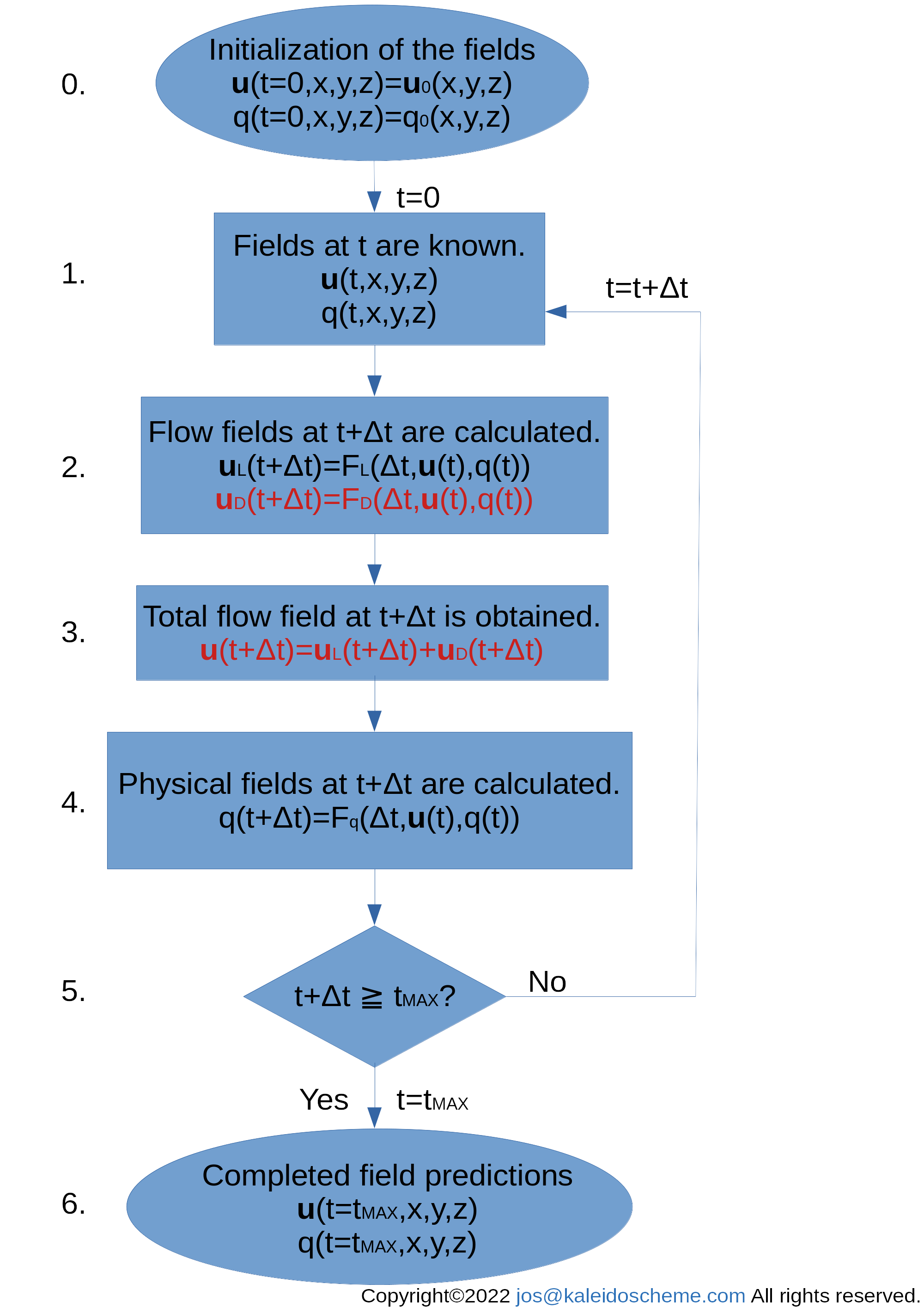
An example of a basic computational procedure of a dynamical detrainment (DD) model. For simplicity of presentation, block 4 is placed in sequence, but it can be calculated independently and in parallel with blocks 2 and 3.
The independent variables t, x, y, and z represent time, latitude, longitude, and altitude in the model, respectively. The three-dimensional velocity field in the atmosphere is denoted as u=(u,v,w). For the sake of illustrating the computational procedure, we assume that the velocity of the atmosphere u is given as the sum u=uL+uD, where uL=(uL,vL,wL) is the velocity field on a large scale obtained explicitly by solving the equation of motion and uD=(uD,vD,wD) is the velocity field given by the dynamical detrainment on a small scale of cumulus clouds. Scalar-valued physical quantities that describe the state of the atmosphere include temperature T, pressure p, density ρ, water vapor mixing ratio qv, etc., all of which are represented by q. All the velocities and physical quantities are calculated, for example, at calculation grid-points (x,y,z) starting from an initial state t=0 and moving forward in time steps of Δt. The calculation is completed when time t reaches the desired prediction time tMAX. The expressions shown in the figure are not mathematically rigorous, but rather illustrate the calculation procedure conceptually. Each block numbered on the left is explained below. Procedures related to dynamical detrainment are indicated by red-colored notations in the blocks.
Calculation Procedure:
(The number at each item corresponds to the number of each block in Fig. 11.)
Flowchart for the RDC scheme
The RDC parameterization will be explained in detail in the next section. For ease of comparison with the calculation procedure of the DD model, here we show the case in which the time step ΔtR for calculating the RDC parameterization FR is the same as the time step Δt for the other calculations FL/FD/Fq. The calculation procedure for taking the time step ΔtR longer than Δt is described separately in "Example of Computational Procedure for a Practical RDC Model" at the end of this page.
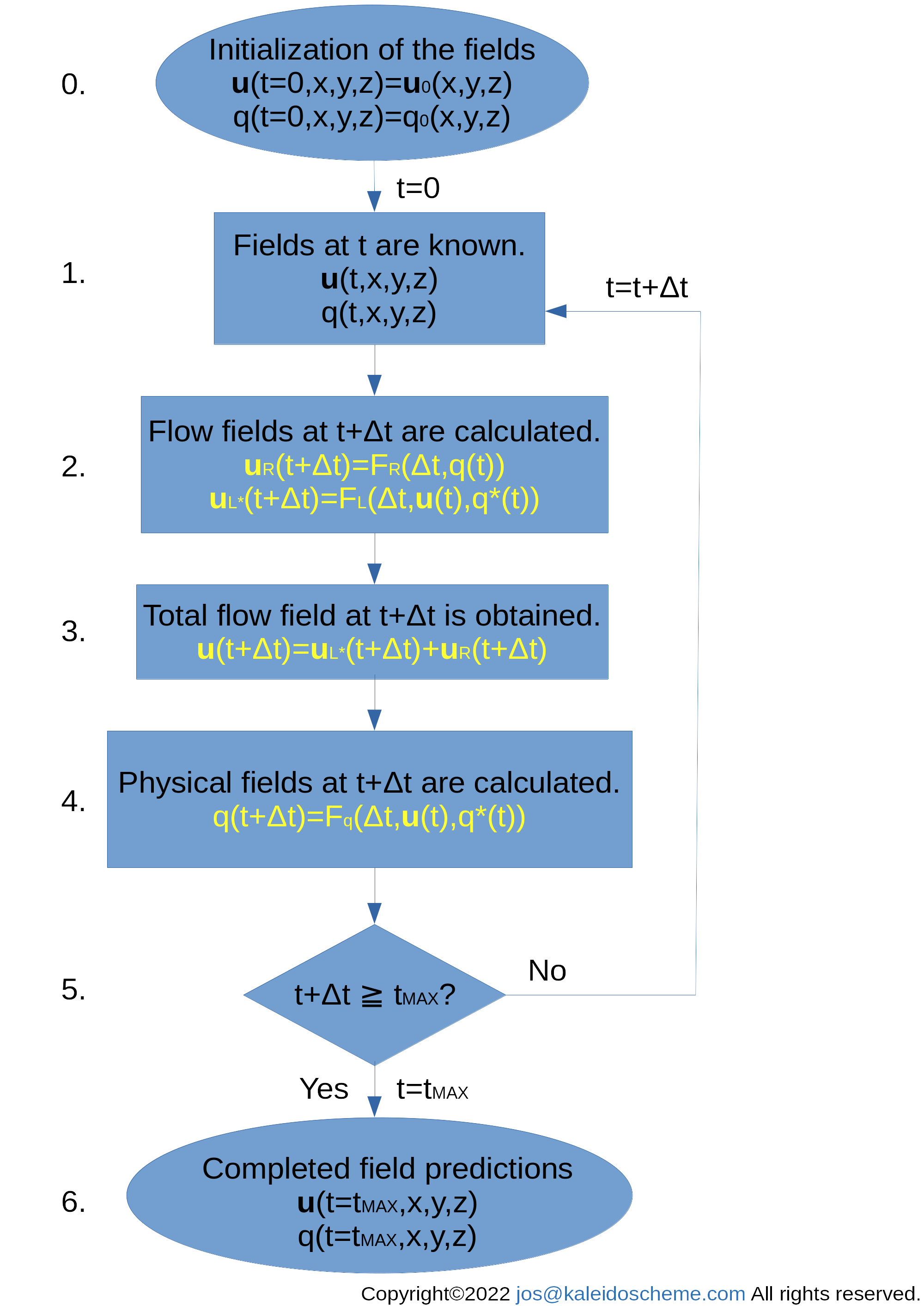
An example of a basic computational procedure of an RDC model. For simplicity of presentation, block 4 is placed in sequence. But it can be calculated independently and in parallel with blocks 2 and 3. For the same reason, the time step ΔtR for calculating the RDC parameterization FR is taken to be the same as the time step Δt for the other calculations FL/FD/Fq. But in practice, ΔtR can be much larger than Δt.
Figure 12. is similar to the dynamical detrainment (DD) model shown in Fig. 11., except for the yellow notations that indicate the procedures involved in the RDC calculations. The most obvious difference is that the velocity field due to dynamical detrainment, represented by uD, is replaced by the velocity field due to RDC, represented by uR.
In the dynamical detrainment (DD) model shown in Fig. 11., the velocity u in the model is expressed as the sum u = uL + uD, where uL is the flow on a large spatial scale and uD is the flow contributed from motion on a small spatial scale. In contrast, we follow the second law of thermodynamics and consider that the atmospheric flow is not affected by the small-scale motion, but is governed only by the large-scale flow. Therefore, the contribution uD from small-scale motion does not appear in the RDC model. Instead, the RDC model considers only flows with large spatial scales and treats them in two categories based on their characteristic time: the "time-averaged component" uR, which has a long characteristic time, and the "disturbance component" uL*, which has a short characteristic time. The velocity u in the model is represented by the sum of them u = uR + uL*. (The "large-scale component" uL in the DD model and the "disturbance component" uL* in the RDC model are velocity components that correspond to each other. But the latter is subscripted with L* in the RDC model instead of L because of some different treatment of the radiative cooling rate.)
In the DD model (Fig. 11.), the equation of motion, which is a differential equation for time, explicitly treats the disturbance component uL of the atmosphere as a dynamical motion, but do not explicitly treat the relationship that the time-averaged component uR of the atmosphere must satisfy. The RDC model extracts and explicitly treats this time-averaged component of the atmosphere uR, which has not been properly treated by the DD model, as the motion required only to maintain thermal equilibrium and continuity in an unforced tropospheric atmosphere. The details of the procedure for calculating the RDC parameterization FR to obtain the RDC velocity uR will be described in the next section.
In the RDC model, the equation of motion
FL
for finding the component
uL*
other than the RDC component
uR,
and the prediction equation
Fq
for finding the physics quantity q,
can be used as used
in the DD model
without modification.
However, the radiative cooling that is eliminated by
uR
no longer has any effect in
the temperature prediction equation
(one of the prediction equations Fq).
Only the radiative cooling that remains unresolved
after
FR
calculation
will be used in
the temperature prediction equation,
on the calculation points other than the points
where the local thermodynamical balance is fully satisfied
by RDC.
To indicate this, in blocks 2. and 4. of Fig. 12.,
the symbol q* is used
for the physical quantity in the arguments in the calculations
FL
and
Fq
to distinguish it from the symbol q used when the radiative cooling rate is used as is.
In blocks 2. and 4.,
when performing calculations where q* appears in the argument,
only the remaining radiative cooling
after being subtracted the amount eliminated by
uR
should be used.
For this purpose, the RDC computation
FR
must precede
the prediction calculations
FL
and
Fq.
(Here we used the general symbol q* both in blocks 2 and 4.
But perhaps the special treatment on q* is needed
only for the radiative cooling rate
used in temperature calculation in block 4.)
[NOTE]
Atmospheric models that explicitly treat the vertical mass flux within the cumulus
should be implemented so that when RDC occurs,
the total horizontal mass outflow through the cumulus flank due to RDC does not
exceed the vertical mass flux available within the cumulus domain.
A Limitation on RDC subsidence mass flux
for this purpose will be discussed in the latter part of this section.
The limitation method will require parameter tuning
by comparing the results with those of the cumulus-resolving model.
When the RDC cannot fully compensate for all radiative cooling
of the surrounding atmosphere
due to insufficient vertical mass flux within the cumulus,
the portion of radiative cooling that remains unresolved
will stay effective on the surrounding atmosphere.
On the other hand,
if the vertical mass flux within the cumulus cloud exceeds
the consumption by the horizontal mass flux of the RDC,
the remaining vertical mass flux is treated by the large-scale dynamics.
Thus,
situations that break the radiative-convective equilibrium
(including cases where the cumulus effect is weak and the atmosphere cools,
and cases where the cumulus effect is strong
to exert forcing on the surrounding atmosphere)
are also correctly represented in the RDC model.
[NOTE]
Conversely,
for atmospheric models that do not provide the vertical mass flux in the cumulus,
it may be possible to determine the vertical mass flux in the cumulus
from the mass flux required by the RDC.
However,
if the RDC-required vertical mass flux within the cumulus is given completely,
the atmosphere outside the cumulus will always be in thermal equilibrium,
and it will not be possible to describe,
for example,
effects such as radiative cooling that destabilize the atmosphere.
Parameter tuning similar to that mentioned in the note above
will be required here again to determine
how much portion of the cumulus mass flux required by RDC should be provided
in the atmospheric model,
in comparison with the results of the corresponding cumulus-resolving model.
[The article continues below.]
"Buffered RDC Method"
An Example of Computational Procedure for a Practical RDC Model
This part addresses technical issues related to practical computation of RDC parameterization.
This example illustrates the so-called "buffered RDC method". That is, if the cumulus mass flux is not sufficient to completely eliminate radiative cooling outside the cumulus cloud, the remaining radiative cooling continues to accumulate, and when the mass flux becomes available, the radiative cooling is removed by lumped sum RDC.
[NOTE]
The Buffered RDC Method shown here is a natural extension
of our previous RDC analysis in the (two-dimensional) time-mean atmosphere
(references)
to the real-time atmosphere.
For example,
for a simple geometry where cumulus clouds develop repeatedly
at only one fixed location in the computational region
and with a sufficiently long accumulation (buffering) time,
the Buffered RDC Method results in an RDC analysis
of the time-mean atmospheric field (but in three-dimensional space this time).
In this case,
the RDC should be fully realized in the atmosphere,
otherwise thermodynamical equilibrium and mass continuity
outside the cumulus cloud cannot be maintained.
Figure 12. showed a flowchart of a simple RDC model when the time interval ΔtR for the RDC calculation is the same as Δt for the dynamics calculation, in order to show the difference from a flowchart of the existing DD model (Fig. 11.). In practice, however, the time step ΔtR can be taken much longer than the time step Δt. This is because the RDC flow is determined by the radiative properties of the atmosphere with a relatively long characteristic time, whereas the other advection calculations are influenced by the dynamical flow with a short characteristic time. Long time steps ΔtR are not only economically advantageous, but also contribute to the numerical stability in the calculation. The physical values used in the RDC parameterization calculation FR are time-mean values averaged over the time step ΔtR. The long time step ΔtR makes these values to have smooth spatial distributions, which stabilize numerical calculations in the RDC parameterization, such as vertical derivatives and horizontal integrations. In exchange, however, a long time interval ΔtR has the disadvantage of delaying the time at which the RDC flow uR is reflected in the model. It is important to find a suitable time interval ΔtR for implementation of RDC parameterization.
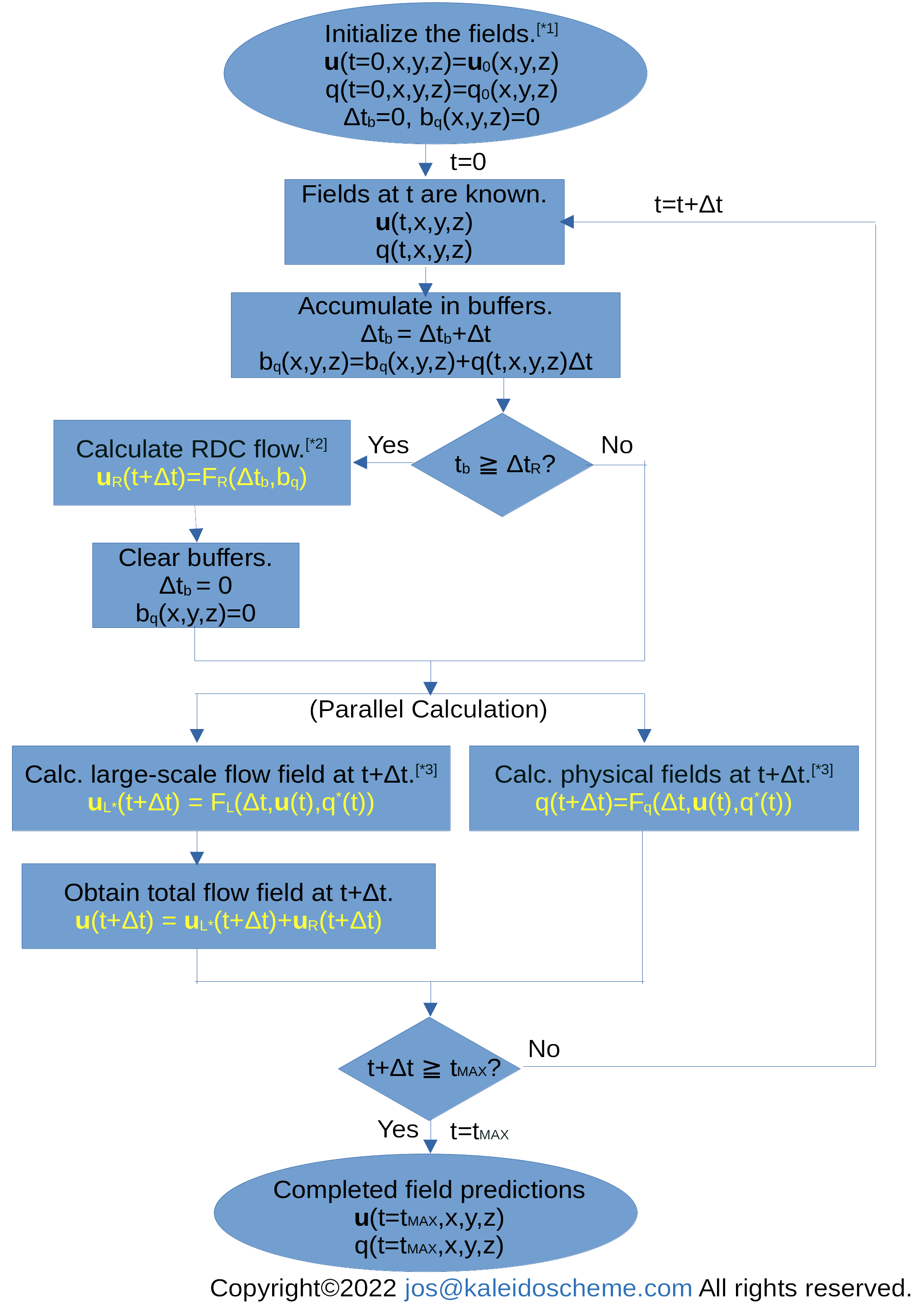
Example of a calculation procedure for a practical RDC model. The time interval ΔtR for the RDC calculation is taken longer than the time interval Δt for the dynamics calculation. And parallel computations are applied to the calculations for the fields of dynamical flow and other physical values. Annotations [*1]-[*3] in the figure are described near the end of this section.
Figure 13. shows an example of a practical RDC model flowchart for the case
ΔtR>Δt.
In this case, physical values q used in the RDC calculation FR
(for example, the vertical mass flux Fmz given by Eq. \eqref{Fmz}
used to calculate the vertical differentiation
in the right-hand side of Eq. \eqref{rdc})
should refer to their time-mean values <q >R
averaged over the time interval ΔtR.
To obtain the time-mean values <q >R of physical values q,
a time accumulator
Δtb
and a set of buffer variables bq
are used:
\begin{eqnarray}
{b}_{q} \left(x,y,z\right)
=
{\int}_{{t}_{\rm{LAST}}}^{{t}_{\rm{LAST}}+\Delta {t}_{b}}
q\left(t,x,y,z\right) dt
\label{buff},
\end{eqnarray}
where tLAST is the time
of the last computation for RDC process.
When the time-mean value
<q>R
of a physical value q
over the time interval ΔtR ≒ Δtb
is required in the RDC calculation
FR,
it can be obtained
by dividing bq by Δtb
as
\begin{eqnarray}
{\langle q \rangle}_{R}
\fallingdotseq
\frac{{b}_{q}}{{\Delta t}_{b}}
\label{mean}.
\end{eqnarray}
[NOTE]
Here we used a nearly-equal symbol ≒ rather than an exactly-equal symbol =.
For example, when severe dynamical motion is expected,
the time step
Δt
for dynamical calculations
may be implemented to take a variable value in order to satisfy
the numerically required Courant condition (CFL condition).
In such a calculation method, the accumulated value in the buffer
Δtb is
not guaranteed to be exactly equal to the specified value
ΔtR
of the time step for RDC calculation.
If atmospheric density ρ is calculated explicitly at each time step Δt in the model, the time-mean density <ρ>R needs to be similarly calculated at every RDC time step ΔtR to obtain the RDC velocity from RDC mass flux as uR =<uR>R =<ρuR>R / <ρ>R.
Furthermore, similar time-mean treatment is required also for radiative cooling rate. Special care should be taken with the radiative cooling rate used for the temperature prediction. Only the portion of radiative cooling rate, which was not eliminated by RDC, should be taken from the time-mean value and used in the temperature prediction equation. (Perhaps the radiative cooling rate is not directly used in other predicting equations.)
Annotations in Fig. 13.
[*1]
During initialization,
the buffer variables tb and bq
must be all zero-cleared.
Since the RDC calculation is not performed during the first time interval ΔtR,
the initial values of the RDC velocity and physical quantities
obtained by the RDC calculation must also be provided.
[*2]
The values used in the RDC calculation are the time-mean values
averaged over the preceding time interval Δtb,
as given by Eq. \eqref{mean}.
Also limiting procedures for the RDC mass fluxes and the RDC radiative cooling rate
(shown by Eqs. \eqref{limitedWR} and \eqref{limitedRadCool})
are performed here.
[*3]
Even when q* appears as an argument in the prediction calculation,
the radiative cooling rate that remains unresolved by
the last RDC calculation FR is used
until the next RDC calculation FR is performed.
[The article continues below.]
RDC Diagnostic Analysis Method for 3D Cumulus-Resolving Atmospheric Models
The computing procedure on this page is presented as the RDC cumulus parameterization method applied to a non-cumulus-resolving model. But it can also be used directly as an RDC analysis method if diagnostically applied to the results of a cumulus-resolving model. Rather than starting parameter tuning as cumulus parameterization in the non-cumulus-resolving model, a practical approach would be to perform RDC diagnostic analysis in a simple cumulus-resolving model with a small region first to confirm that the RDC mechanism actually works in a three-dimensional time-developing atmospheric model. The RDC diagnostic analysis will also provide information used in RDC parameter-tuning in the non-cumulus-resolving model, such as a suitable time interval ΔtR between the RDC computations, an appropriate condition for designation of the supplying source domains, and the limiting constant/function L1i. Thus, the RDC parameter-tuning will be performed in comparing the RDC diagnostic analysis on the atmosphere obtained from the cumulus-resolving model with the RDC parameterization being constructed in the non-cumulus-resolving model. Such a method would allow comparing only the RDC components between the cumulus-resolving and non-cumulus-resolving models. The parameter tuning based on RDC, which has a solid physical basis described on this page, would be easier than that for DD.
More to the point, you don't even need a cloud-resolving model. The RDC diagnostic analysis method can be used with a non-cumulus-resolving model, as long as it can clearly distinguish cumulus-bearing domains from other clear-sky regions. Although a supplying source domain may not correspond exactly to an individual cumulus cloud, it should still be possible to show that the RDC flow field is what should be present in the model atmosphere. And the RDC flows from the supplying source domains will be shown to involve much more efficient transport of mass, heat, and water vapor than the flows of any existing dynamic detrainment method. This analysis appears to be the easiest one for most people to start with.
[NOTE]
In the case of non-cumulus-resolving models, however,
the flow around the cumulus cloud obtained by RDC analysis
shows the flow which is required in the atmosphere.
This may differ from the flow around the cumulus
given by the parameterisation actually implemented in the model.
This difference will show how far the cumulus parameterisation currently used in the model
differs from what is actually required.
The crucial final addition is that the RDC analysis to show the validity of the RDC transport is enough to be done only once. You get the average state of the equilibrium atmosphere over a single time interval from a 3D atmospheric model, and you only need to apply the RDC analysis to that field once to get the result. This means that you do not need to incorporate the RDC analysis code into the atmospheric model. You simply feed the mean-field physical data output from the atmospheric model into a boundary value problem solver outside the model. For these early attempts with RDC analysis, a very simple framework is preferred. That is, a rough estimate, without the detailed tuning described above, would show the essence of RDC; applying the boundary value problem of Eq. (\ref{poisson}) to the whole atmosphere without partitioning the horizontal domain, and ignoring the constraints on the RDC flow required by the vertical mass fluxes in the cumulus cloud.
[NOTE]
A general procedure for the RDC Diagnostic Analysis:
-
[NOTE]
Some researchers may find it tedious to solve the Poisson equation (\ref{poisson}) at the end of the RDC analysis procedure. As a very first evaluation, you can get a rough idea of the flow field just by looking at the distribution of values on the right-hand side of Eq. (\ref{poisson}) (or the basic RDC equation (\ref{rdc})) at a height together with the locations of supplying source (cumulus) domains, without rigorously solving the Poisson equation.
External Parameters
Although most computations in the RDC scheme are determined based on fundamental physical laws, there are a few that cannot be determined solely from the physical processes of RDC.
Our Current Consideration Regarding the RDC Calculation Interval tR (2025/10/01)
Some of you may have noticed a delay in the reflection of atmospheric conditions in RDC calculations. In order to achieve smooth distributions of the RDC data (values of the variables appearing on the right-hand side of the RDC Poisson equation \eqref{poisson}, namely, density, temperature lapse rate, and radiative cooling rate), the calculation must use the data averaged over a time interval tR that is larger than the typical timescale of dynamical disturbances, such as the lifetime of cumulus clouds. However, this approach cannot resolve the temporal development of cumulus clouds. Simply shortening tR, to see the contribution at each stage of cumulus development, prevents the removal of dynamical disturbances. This forces us to partition the horizontal area and to solve the RDC boundary value problems, using a disturbed field of the data distribution. And finally, this may make it difficult for each calculation to converge numerically.Our current approach to this problem is as follows: When tR is shortened to resolve the developmental stages of cumulus clouds, before the RDC computations, not only we will average the data distribution TEMPORALLY over tR, but also we will smooth it SPATIALLY. This preprocessed data field, both temporally and spatially smoothed, allows us to partition the horizontal area and to solve the RDC boundary value problems stably. Worried about the contribution lost from fine structures due to smoothing? Don't worry. The portion obtained by subtracting the smoothed RDC component from the entire model variable corresponds to the disturbance component. This is passed to the model's equations of motion and handled dynamically. Even if there are excess or insufficient parts in the RDC flow, the dynamical flow should adjust it, by removing or supplementing them. Consequently, this approach should ultimately yield consistent results.
Theoretically, this method seems to work, but of course, it should be actually confirmed within a 3D model if the RDC flow is properly represented.
Summary
As you can see from all the explanations on this site, it is clear that RDC is an essential process in an equilibrium atmosphere and is responsible for effective mass, heat, and water vapor transport. We believe that even a non-rigorous RDC diagnostic analysis as the first step verification will demonstrate the validity and the transport efficiency of the RDC flow. We hope that as many researchers as possible will try this RDC diagnostic analysis as a starting point for RDC.
Thanks for reading the long explanation.
But this is still not enough,
so please examine
Brief Considerations on RDC
and
References.
All rights of the RDC scheme
(including the cumulus parameterization and
the corresponding 3D diagnostic analysis method),
its variants,
and the subtheories and subtechnologies
(i.e., theories and technologies assuming the RDC scheme,
whether or not they are described here),
as well as all the articles on this website,
are owned exclusively by jos <jos@kaleidoscheme.com>
the author of this website.
The development or assertion of any related theory and technology
that would limit the Owner’s right
to distribute or commercialize the RDC scheme is strictly prohibited.
The RDC scheme must remain free from any third-party encumbrances
that prevent its independent distribution, licensing, or sale.
The RDC scheme is a product of
Kaleidoscheme,
who is entrusted with all management of
user contracts and copyright protection.
You are prohibited from using (i.e., quoting, implementing, and operating)
the RDC scheme
without an agreement with
Kaleidoscheme.
No one may use the RDC scheme without a contract with us.
An agreement is required, except for internal reviews by individuals or organizations,
and direct communication with us.
This is especially important for external publications.
It ensures that the value of the RDC scheme is not diminished
by misuse from those who do not understand it.
We will address any misunderstandings or misuse of the RDC scheme.
The flowcharts and program codes listed on this website are all examples,
as it is impossible to enumerate every case.
Although plenty of variants are possible,
any citation, implementation, or operation based on the RDC scheme
is prohibited without agreement with us.
The contract for the right to use the RDC scheme must be concluded
at the time the development is initiated,
so that we can correct your misunderstandings and misuse
at the earliest possible stage.
The contents on this website will be updated irregularly
when the author finds errors or incomplete descriptions.
Thank you for your understanding.
RDC Parameterization < rdctheory.cloud
Contact Us
Exhibited on 2022/07/30
Last updated on 2026/06/13
Copyright(C)2022-2026 jos <jos@kaleidoscheme.com> All rights reserved.